BiostatR Blog

Adapted from  https://ryanhomer.github.io/posts/build-openmp-macos-catalina-complete Install R from  cran.r-project.org At the end of ~/.zshrc add:  export PATH=$PATH:/Library/Frameworks/R.framework/Versions/Current/Resources/bin/ Then you can use R within the terminal. Install macbrew via: /bin/bash -c "$(curl -fsSL https://raw.githubusercontent.com/Homebrew/install/HEAD/install.sh)" Then in ~/.Rprofile: marcgirondot@MacBook-Pro-de-Marc ~ % cat .Rprofile # Default CRAN mirror options(repos=structure(c(CRAN="https://cloud.r-project.org/"))) # Path to run R with system Sys.setenv(PATH=paste(Sys.getenv("PATH"), "/Library/Frameworks/R.framework/Versions/Current/Resources/bin/", sep=":")) Install llvm brew install llvm libomp Install GCC and gettext brew install gcc gettext To configure R to build packages with the versions of clang and gcc you just installed, set up a Makevars file. This must be located at ~/.r/Makevars. Some parts do no w

The Hessian matrix at a point P (P is a vector) is the matrix of partial derivatives at this point. It is often used after non-linear optimization and the standard error of parameters can be obtained using the square-root of the diagonal of the inverse of the Hessian matrix. But when you are estimate SE like this, you lost the covariances between parameters. Then if you estimate random numbers using the SE of parameters, the original structure is lost. It is much better to estimate random numbers directly from the Hessian matrix. Then you keep the variance-covariance structure. When the model is fitted using MCMC, no Hessian matrix is directly available. A pseudo-Hessian matrix can be calculated using: hessian <- solve(cov( [matrix of values for different iterations] )) Let do an example with the fit of a normal distribution: First using maximum likelihood: val <- rnorm(30, 10, 2) library(MASS) ft <- fitdistr(val, densfun="normal") The Hessian matrix is not available

Let create two variables of length 100, one with mean 10 (A) and one with mean 12 (B) both with SD=2. Of course the two variables overlap. A <- rnorm(100, 10, 2) B <- rnorm(100, 12, 2) library(HelpersMG) barplot_errbar(c(mean(A) ,mean(B)), errbar.y = c(1.96*sd(A), 1.96*sd(B)), las=1, ylim=c(0, 20), main="1.96 x SD") Now do a t test. It is highly significant: t.test(A, B) Welch Two Sample t-test data:  A and B t = -7.8344, df = 197.93, p-value = 2.82e-13 alternative hypothesis: true difference in means is not equal to 0 95 percent confidence interval:  -2.737632 -1.636588 sample estimates: mean of x mean of y   9.741912 11.929021  Then if you want use the overall of confidence interval, use SE: barplot_errbar(c(mean(A) ,mean(B)), errbar.y = c(1.96*sd(A)/sqrt(length(A)),   1.96*sd(B)/sqrt(length(A))), las=1, ylim=c(0, 12), main="1.96 x SE")

The conclusion is that it artificially reduced the variability of the correlation coefficient. It is bad practice. But it is much better than doing nothing ! cor.original <- NULL cor.na <- NULL cor.median <- NULL for (i in 1:10000) {   A <- rnorm(100, mean=100, sd=20)   B <- rnorm(100, mean=100, sd=20)   Bprime <- ifelse(sample(c(0,1), 100, replace = TRUE), B, NA)   Bter <- ifelse(is.na(Bprime), median(B, na.rm = TRUE), Bprime)   cor.original <- c(cor.original, cor(x=A, y=B, method = "spearman"))   cor.na <- c(cor.na, cor(x=A, y=Bprime, method = "spearman", use="complete.obs"))   cor.median <- c(cor.median, cor(x=A, y=Bter, method = "spearman", use="complete.obs")) } layout(1:3) hist(cor.original, xlim=c(-0.6, 0.6), breaks=seq(from=-0.6, to=0.6, by=0.05)) hist(cor.na, xlim=c(-0.6, 0.6), breaks=seq(from=-0.6, to=0.6, by=0.05)) hist(cor.median, xlim=c(-0.6, 0.6), breaks=seq(from=-0.6, to=0.6, by=0.05)) quanti

 It is better to supply a initial point for robust regression ! x <- c(0.428571428571429, 0.2, 0.3, 0, 0, 0.2, 0, 0, 0.1, 0, 0.1,    0.1, 0, 0, 0, 0.3, 0.2, 0.3, 0.2, 0.2, 0, 0, 0, 0.2, 0.222222222222222,    0.1, 0, 0.4, 0.3, 0.5, 0, 0.4, 0.5, 0.8, 0.3, 0.1, 0.2, 0, 0.1,    0, 0.1, 0.1, 0.4, 0, 0, 0, 0, 0, 0, 0.333333333333333, 0.444444444444444,    0.2, 0.222222222222222, 0, 0, 0, 0, 0, 0, 0, 0, 0, 0, 0, 0, 0,    0, 0, 0, 0, 0.4, 0, 0, 0, 0, 0.111111111111111, 0, 0, 0, 0, 0,    0, 0, 0, 0, 0, 0, 0, 0, 0, 0, 0, 0, 0, 0, 0, 0, 0, 0, 0, 0, 0,    0, 0, 0, 0, 0, 0, 0, 0, 0, 0, 0, 0, 0, 0, 0, 0, 0, 0, 0, 0, 0,    0.5, 0, 0, 0, 0, 0, 0, 0, 0, 0, 1, 0.2, 0, 0, 0, 0, 0, 0, 0) y <- c(0.369999388816617, 0.152260672623962, 0.392636473518975, 0.107742543910461,         0.105802942749025, 0.147888875829182, 0.0180958542177892, 0.00376865991773073,         0.00852273837059186, 0.00857162539273257, 0.112051915806605,         0.0755798935035902, 0.0268356635188166, 0.00419682981147497,         0

Often I want create a named vector and the names are stored in a variable. I must use a 2 steps function: names <- paste0("V", 1:100) A <- 1:100 names(A) <- names I search a way to do the same in a single step. Here is the solution: A <- structure(1:100, .Dim = 100L,                     .Dimnames = list(names)) But which one is the faster? names <- paste0("V", 1:100) library(microbenchmark) microbenchmark({     A <- 1:100     names(A) <- names},      {A <- structure(1:100, .Dim = 100L,                     .Dimnames = list(names))},      times = 1000L) Unit: microseconds                                                                 expr  min    lq     mean                             {     A <- 1:100     names(A) <- names } 1.02 1.068 1.222658  {     A <- structure(1:100, .Dim = 100L, .Dimnames = list(names)) } 5.78 6.295 6.486045  median     uq    max neval cld  1.2475 1.3310  4.658  1000  a   6.4090 6.5575 33.790  1000   b In conc

Let use the same nc file obtained from NOAA ( http://www.esrl.noaa.gov/psd/data/gridded/data.noaa.oisst.v2.highres.html ) be used. Here I show the 3 ways to get annual data depending on the package used. In conclusion, RnetCDF does not scale data using scale_factor and add_offset automatically. Take care. utcal.nc from package RnetCDF is very useful. dest <- "sst.day.mean.2014.v2.nc" For all the package, I will use the same coordinates: lat=35, lon=28 # Note that the function ind_long_lat can be used data from any of these packages library(RNetCDF) dat.RNetCDF <- open.nc(dest) lat=35 lon=28 # it will be used for all data library(phenology) indice <- ind_long_lat(ncdf=dat.RNetCDF, long=lon, lat=lat) Packages RnetCDF # take care, it does not scale automatically the data point_SST.RNetCDF_wrong <- var.get.nc(ncfile=dat.RNetCDF, variable="sst",                                  start=c(indice ,1), count=c(1, 1, 1)) # correct method point_SST.RNetCDF_corr <

Just add \\ at the position of return \documentclass[a4paper]{article} \usepackage[utf8]{inputenc} \begin{document} \tableofcontents \section{Essai\\Pour un titre} <<>>= degree <- "o" print(degree) @ \end{document}

If you need fit a probability using optim(), it is more secure to fit an inverse logit value and use a logit transformation after to ensure that the values stay always between 0 and 1: L <- c(1.2) p <- 1/(1+exp(L)) And then the probabilities of the two events are p and 1-p. However it is more difficult in the case of multinomial distribution because the sum of the probabilities must be 1. Here is the correct way to do. For N events, you need N-1 parameters: L <- c(10, -1, 3, 7, 0) p <- 1/(1+exp(L)) p [1] 4.539787e-05 7.310586e-01 4.742587e-02 9.110512e-04 5.000000e-01 The trick is to transform these probabilities into conditional probabilities: p.multinomial <- function(p) c(p, 1)*c(1, sapply(seq_along(p), function(i) prod(1-p[1:i]))) p.multinomial(p) [1] 4.539787e-05 7.310254e-01 1.275420e-02 2.333885e-04 1.279708e-01 1.279708e-01 sum(c(p, 1)*c(1, sapply(seq_along(p), function(i) prod(1-p[1:i])))) [1] 1 To do the reverse: inv.p.multinomial <- f

save.image(file= " xxx.Rdata") save the content of memory to be reused, but it does not work within a function. There, you can use: save(list = ls(all.names = TRUE), file = "total.Rdata", envir = environment()) For example: essai <- function(x) {   blabla <- c("ldklklkdlkd")   save(list = ls(all.names = TRUE), file = "total.Rdata", envir = environment()) } load("total.Rdata")

# generate data jo <- 1:800 trans_trigo <- 10+sin((jo/365.25)*2*pi)*1+ cos((jo/365.25)*2*pi)*5 obs <- rnorm(n=800, mean=trans_trigo, sd=2) # plot the data plot(jo, obs, bty="n", xlim=c(1,800), ylim=c(0,20)) par(new=TRUE) plot(jo, trans_trigo, bty="n", xlim=c(1,800), ylim=c(0,20), xlab="", ylab="",      axes=FALSE, col="violet", type="l", lwd=2) # group is per month observation mydat <- data.frame(obs=obs, jour=jo, jour2=jo*jo, group=round(jo/27)) # glm with ordinal day as linear factor mod <- glm(obs ~ jour, data=mydat, family=gaussian) summary(mod) newdata <- data.frame(jour=1:800) preddf2 <- predict(mod, type="response", newdata=newdata, se.fit=FALSE) par(new=TRUE) plot(jo, preddf2, bty="n", xlim=c(1,800),  ylim=c(0,20), xlab="", ylab="", axes=FALSE, col="red", type="l") # glm with ordinal day as second degree polynom mod3

brew reinstall openssl@1.1 wget https://cran.r-project.org/src/contrib/openssl_1.4.2.tar.gz R CMD INSTALL --configure-vars='INCLUDE_DIR=/usr/local/opt/openssl@1.1/include LIB_DIR=/usr/local/opt/openssl@1.1/lib' openssl_1.4.2.tar.gz

I had an error when I tried to update rgdal. It said that gdal 2.1.4 was installed whereas brew installed version 3.1 The 2.1.4 version was installed previously manually in : /Library/Frameworks I remove the gdal folder, installed gdal using brew and all is ok now: brew install gdal and in R: install.packages("rgdal") Note that rgdal should be replaced by terra in future

echo $USER will show your login name; for example myname Then do: sudo chmod -R 777 /Users/myname/Library/R/4.0/library/ and you will be able to install packages within RStudio

# Install Ubuntu 20.04 lts # 2 hours sudo apt install update-manager-core sudo apt update sudo apt upgrade sudo apt dist-upgrade sudo apt autoremove sudo reboot sudo do-release-upgrade -d # Remove old R installation # If you want install again your packages, follow this trick #  https://biostatsr.blogspot.com/2019/05/reinstall-packages-after-updating-r.html sudo vi /etc/apt/sources.list # Remove all lines with CRAN or r-project # In vi, use / to search # Remove files shown using: ls /etc/apt/sources.list.d # For example: sudo rm /etc/apt/sources.list.d/marutter-ubuntu-rrutter3_5-xenial.list sudo rm /etc/apt/sources.list.d/marutter-ubuntu-rrutter3_5-xenial.list.distUpgrade sudo rm /etc/apt/sources.list.d/marutter-ubuntu-rrutter3_5-xenial.list.save # I am not sure that reboot is necessary, but better to do! sudo reboot sudo apt-get purge r-base* r-recommended r-cran-* sudo apt autoremove sudo apt update # Packages are located in .libPaths() read from

In terminal: sudo apt-get update -y sudo apt-get install -y fftw3 In R install.packages("imager") More infos here: http://dahtah.github.io/imager/ In MacOSX:  brew install imagemagick ffmpeg Note: imagemagick@6 is keg-only, which means it was not symlinked into /usr/local, because this is an alternate version of another formula. If you need to have imagemagick@6 first in your PATH, run:   echo 'export PATH="/usr/local/opt/imagemagick@6/bin:$PATH"' >> ~/.zshrc For compilers to find imagemagick@6 you may need to set:   export LDFLAGS="-L/usr/local/opt/imagemagick@6/lib"   export CPPFLAGS="-I/usr/local/opt/imagemagick@6/include" For pkg-config to find imagemagick@6 you may need to set:   export PKG_CONFIG_PATH="/usr/local/opt/imagemagick@6/lib/pkgconfig"

Sometimes it is not possible to use only ASCII character and it prevents to pass the CRAN check. For example, if you need to use "−"; clearly it will generate an error in the CRAN check. The solution is to use the chr() and asc() functions of my HelpersMG package available in CRAN: Do: > asc("−") [1] 195 162 203 134 226 128 153 And replace "−" in your code by: > chr(c(195, 162, 203, 134, 226, 128, 153)) [1] "−" You will have the magic message: Status: OK after your check for CRAN! https://cran.r-project.org/web/packages/HelpersMG/index.html

df <- data.frame(Fibro=sample(x=c("Oui", "Non"), 1000, replace=TRUE),                  year=floor(runif(1000, min=2004, max=2010))-2000,                  ID=sample(x=1:100, 1000, replace=TRUE)) df2 <- cbind(df, FibroNum=as.numeric(df$Fibro=="Oui"), NonFibroNum=1-as.numeric(df$Fibro=="Oui")) df2$year <- df2$year + df2$FibroNum df2$Fibro <- as.factor(df2$Fibro) df2$ID <- as.factor(df2$ID) head(df2) library(lme4) These solutions are equivalent g1 <- glmer(formula = Fibro ~ year + (1 | ID), data=df2, family=binomial(link="logit")) g2 <- glmer(formula = FibroNum ~ year + (1 | ID), data=df2, family=binomial(link="logit")) g3 <- glmer(formula = cbind(FibroNum, NonFibroNum) ~ year + (1 | ID),             data=df2, family=binomial(link="logit")) library(cAIC4) cAIC(g1) cAIC(g2) cAIC(g3)

The prior for proportion should be chosen within Beta distribution.  Beta distribution in Wikipedia Beta distribution has two parameters, alpha and beta (alpha>0 and beta>0) and it used a parameter 0≤x≤1. x can be a proportion. For such a reason, Beta distribution is perfect to be used as a prior for proportion. Look at the shape of beta: colors = c("red","blue","green","orange","purple", "black") grid = seq(0,1,.01) alpha = c(.5,5,1,2,2, 1) beta = c(.5,1,3,2,5, 1) plot(grid,grid,type="n",xlim=c(0,1),ylim=c(0,4),xlab="",ylab="Prior Density",      main="Prior Distributions", las=1) for(i in 1:length(alpha)){   prior = dbeta(grid,alpha[i],beta[i])   lines(grid,prior,col=colors[i],lwd=2) } legend("topleft", legend=c("Beta(0.5,0.5)", "Beta(5,1)", "Beta(1,3)", "Beta(2,2)", "Beta(2,5)", "Beta(1,1)"),

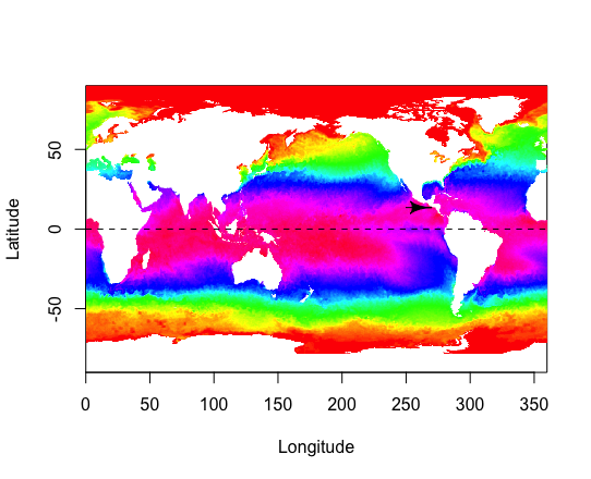
library("HelpersMG") # Guatemala map # get the ncdf file here for 2010, 2011, 2012 # <a href="http://www.esrl.noaa.gov/psd/cgi-bin/db_search/DBListFiles.pl?did=132&tid=33865&vid=2423">http://www.esrl.noaa.gov/psd/cgi-bin/db_search/DBListFiles.pl?did=132&tid=33865&vid=2423</a> # ftp://ftp.cdc.noaa.gov/Datasets/noaa.oisst.v2.highres/sst.day.mean.2012.v2.nc # ftp://ftp.cdc.noaa.gov/Datasets/noaa.oisst.v2.highres/sst.day.mean.2011.v2.nc # ftp://ftp.cdc.noaa.gov/Datasets/noaa.oisst.v2.highres/sst.day.mean.2010.v2.nc url <- "ftp://ftp.cdc.noaa.gov/Datasets/noaa.oisst.v2.highres/sst.day.mean.2012.v2.nc" dest <- paste(Sys.getenv("HOME"), "/sst.day.mean.2012.v2.nc", sep="") download.file(url, dest) url <- "ftp://ftp.cdc.noaa.gov/Datasets/noaa.oisst.v2.highres/sst.day.mean.2011.v2.nc" dest <- paste(Sys.getenv("HOME"), "/sst.day.mean.2011.v2.nc",

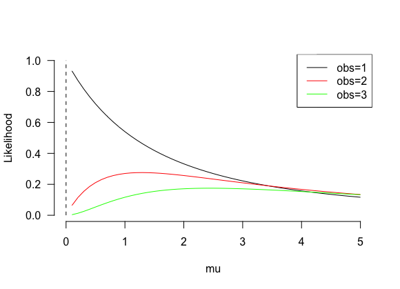
First, let try a NB distribution with mu and theta: mu <- 3; theta <- 2.4 d <- NULL; for (i in 0:20) d <- c(d, dnbinom(i, size=theta, mu=3, log=FALSE)) sum(d) The sum of probability mass functions is 1. All is perfect. Let do a zero-truncated negative binomial distribution after Girondot M (2010) Editorial: The zero counts. Marine Turtle Newsletter 129: 5-6  e <- d[-1]/(1-d[1]) sum(e) The sum of probability mass functions is 1. All is perfect again. Let estimate the likelihood of observations when mu varies. The idea is to check what mu value will be selected using optim() obs <- 1 f <- NULL s <- seq(from=0, to=5, by=0.1) for (mu in s)   f <- c(f , dnbinom(obs, size=theta, mu=mu, log=FALSE)/(1-dnbinom(0, size=theta, mu=mu, log=FALSE))) plot(s, f, type="l", bty="n", las=1, ylim=c(0, 1), xlab="mu", ylab="Likelihood") obs <- 2 f <- NULL s <- seq(from=0, to=5, by=0.1) for (mu in s)   f <

Let do: > as.character(as.Date("2020-06-07"), format="%d/%m/%y") [1] "07/06/20" But what to do if you want just 7/6/20 ? Here is the solution: > gsub("^0", "", gsub("([-])0", "\\1", as.character(as.Date("2020-06-07"), format="%d/%m/%y"))) [1] "7/06/20" Or > d <- as.character(as.Date("2020-06-07"), format="%d/%m/%y") > gsub("^0", "", gsub("/0", "/", d)) [1] "7/6/20"

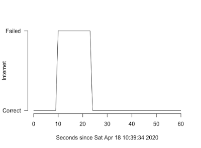
library("beepr", "curl") internet <- NULL TimeToMonitorInSeconds <- 60 # 60*60*5 plot(0:TimeToMonitorInSeconds, rep(0, 1+TimeToMonitorInSeconds), xlim=c(0, TimeToMonitorInSeconds),      ylim=c(0, 1), type="n", bty="n",      xlab=paste0("Seconds since ", date()), ylab="Internet", yaxt="n", xaxt="n") axis(1, 0:TimeToMonitorInSeconds) axis(2, c(0, 1), labels = c("Correct", "Failed"), las=1) previousx <- NULL previousy <- NULL for (i in 0:TimeToMonitorInSeconds) {   t <- curl::has_internet()   names(t) <- date()   # print(t)   if (!t) beep()   internet <- c(internet, t)   if (!is.null(previousx)) segments(x0=previousx, x1=i, y0=previousy, y1=ifelse(t, 0, 1))   previousx <- i   previousy <- ifelse(t, 0, 1)   Sys.sleep(1) } # General plot plot(0:TimeToMonitorInSeconds, ifelse(internet, 0, 1), ylim=c(0, 1), type="l", bty="n&q

df <- data.frame(length=1:100,                  year=c(rep(1980, 20), rep(1981, 20), rep(1983, 20), rep(1984, 20), rep(1985, 20))) boxplot(length ~ year, df) # Not good ! df$year <- factor(df$year,  levels = 1980:1985) boxplot(length ~ year, df)

In terminal: brew install libxml2 wget https://cran.r-project.org/src/contrib/xml2_1.2.5.tar.gz (check the latest version here:  https://cran.r-project.org/web/packages/xml2/index.html ) R CMD INSTALL --configure-vars='INCLUDE_DIR=/usr/local/opt/libxml2/include/libxml2 LIB_DIR=/usr/local/opt/libxml2/lib/' ./xml2_1.2.5.tar.gz

To update the  nloptr  package, you need do first: brew install nlopt in terminal

library(imager) # Ici l'image est en couleur car chaque pixel a 3 valeurs: Red Green Blue (RGB) a <- array(data = runif(10*10*1*3), dim=c(10, 10, 1, 3)) class(a) <- c("cimg", "imager_array", "numeric") plot(a) print.default(a) # Ici l'image est en niveau de gris car on met la même valeur pour RGB a <- array(data = rep(runif(10*10*1), 3), dim=c(10, 10, 1, 3)) class(a) <- c("cimg", "imager_array", "numeric") plot(a) print.default(a) # I add a red point a[5, 5, 1, 1:3] <- c(1, 0, 0) plot(a, interpolate = FALSE) # Ici je ne garde qu'une valeur au lieu de 3 pour RGB; c'est donc du niveau de gris a <- a[, , , 1, drop=FALSE] plot(a) print.default(a) # là je seuille les valeurs a[, , 1, 1] <- ifelse(a[, , 1, 1]<0.5, 0, 1) plot(a) print.default(a)

Let this python code to be parallelized: import time def basic_func(x):     if x == 0:         return 'zero'     elif x%2 == 0:         return 'even'     else:         return 'odd'      starttime = time.time() for i in range(0,10):     y = i*i     # time.sleep(2)     print('{} squared results in a/an {} number'.format(i, basic_func(y)))      print('That took {} seconds'.format(time.time() - starttime)) Do this in R: library(microbenchmark) library(parallel) microbenchmark({out1 <- parallel::mclapply(1:1000, FUN=function(x) {system("python3 essai.py", intern=TRUE)}, mc.cores = detectCores())}, times = 1L) microbenchmark({out1 <- lapply(1:1000, FUN=function(x) {system("python3 essai.py", intern=TRUE)})}, times = 1L)

lme4ord package is available in GitHub but cannot be installed due to an error: > library(remotes) > install_github("stevencarlislewalker/lme4ord") Downloading GitHub repo stevencarlislewalker/lme4ord@master Installing 1 packages: ape essai de l'URL 'https://cran.rstudio.com/bin/macosx/el-capitan/contrib/3.6/ape_5.3.tgz' Content type 'application/x-gzip' length 2612810 bytes (2.5 MB) ================================================== downloaded 2.5 MB The downloaded binary packages are in /var/folders/1v/rfxtzxc11kj33kb8tg7znw080000gn/T//RtmprjveC6/downloaded_packages ✓  checking for file ‘/private/var/folders/1v/rfxtzxc11kj33kb8tg7znw080000gn/T/RtmprjveC6/remotesda0d258c4827/stevencarlislewalker-lme4ord-5f62664/DESCRIPTION’ (471ms) ─  preparing ‘lme4ord’: ✓  checking DESCRIPTION meta-information ... ─  checking for LF line-endings in source and make files and shell scripts ─  checking for empty or unneeded directories ─  building

I have not found a method to estimate confidence interval of orthogonal regression. Then I build one using bootstrap. OrthogonalRegression <- function(x, y) {   library("pracma")   xnew <- seq(from=min(x), to=max(x), length.out = 100)   replicate <- 1000   m <- matrix(data=NA, nrow=replicate, ncol=length(xnew))   c <- NULL   d <- NULL   odrx <- odregress(x, y)   for (r in 1:replicate) {     s <- sample(1:length(x), length(x), replace = TRUE)     odr <- odregress(x[s], y[s])     cc <- odr$coeff     c <- c(c, cc[1])     d <- c(d, cc[2])     # Prediction     ynew <- cbind(xnew, 1) %*% cc     m[r, ] <- ynew   }   q <- apply(m, MARGIN=2, FUN=quantile, probs=c(0.025, 0.5, 0.975))   q <- rbind(q, x=xnew)   qb <- quantile(c, probs=c(0.025, 0.5, 0.975))   qa <- quantile(d, probs=c(0.025, 0.5, 0.975))     return(list(model=odrx,               values=q,               intercept=qa,               slope=qb))

The pch=19 is a circle and secondary plain circle. The pch=16 is only a plain circle. This is what to use for transparency. plot(rep(1, 10) ,rep(1, 10), pch=19, cex=10, col=rgb(.1, .1, .1, 0.01), lwd=5) plot(rep(1, 10) ,rep(1, 10), pch=16, cex=10, col=rgb(.1, .1, .1, 0.01), lwd=5)