BiostatR Blog

Here is a function to implement broken y-axis. Several enhancements could be done to make it nicer but it works. However it was not fully tested.

Let try different solutions to mimic C operand ++ to have the most efficient.

Sometimes you must remove names of elements within a vector. The most classic way to do is to use unname() function. However, the use of as.numeric() or as.character() is more efficient if you know the content of the vector. In conclusion, to remove names, it is 5 times more rapid to use as.integer(), as.character(), as.numeric() or as.logical(). i <- c(Pi=pi) system.time(for (j in 1:100000) k <- unname(i)) utilisateur     système      écoulé        0.171       0.002       0.174  system.time(for (j in 1:100000) k <- as.numeric(i)) utilisateur     système      écoulé        0.030       0.000       0.029    i <- c(Pi=3) system.time(for (j in 1:100000) k <- unname(i)) utilisateur     système      écoulé        0.169       0.003       0.174  system.time(for (j in 1:100000) k <- as.integer(i)) utilisateur     système      écoulé        0.028       0.000       0.028    i <- c(Pi="pi") system.time(for (j in 1:100000) k <- unname(i)) utilisateur    

In a previous post ( http://biostatsr.blogspot.fr/2016/02/comparison-of-methods-to-concatenate.html ), I showed that the use of c <- c(c, x) for concatenation was not efficient at all. Now I study if the efficiency depends on the length of the c object. Vector c <- NULL t <- NULL for (j in 1:40) {     t <- c(t, system.time(         for (i in 1:1000) c <- c(c, pi)     )[1])      } plot(1:40, t, bty="n", las=1, ylim=c(0, 0.4), xlim=c(1, 40)) And the answer is clearly: YES ! The longer the vector c is, the more time it takes to add a new element. And this effect is of course not observed if replacement inside a vector object is done. Note that the y-scales are not the same. c <- rep(NA, 40000) t <- NULL for (j in 1:40) {     t <- c(t, system.time(         for (i in 1:1000) c[(j-1)*40+i] <- pi     )[1])      } plot(1:40, t, bty="n", las=1, ylim=c(0, 0.005), xlim=c(1, 40)) Or better: c <- rep(NA, 40

A symmetric matrix can be useful is many context and it is good to be able to generate such a matrix. Here are several solutions. The most complete function was  symmetricize()  available in the discontinuited package ENA. I copy the function from this package to my package HelpersMG to make it again available: Matrix library > library(Matrix) > essai <- matrix(data = 1:25, nrow = 5) > > forceSymmetric(x=essai, uplo="U") 5 x 5 Matrix of class "dsyMatrix" [,1] [,2] [,3] [,4] [,5] [1,] 1 6 11 16 21 [2,] 6 7 12 17 22 [3,] 11 12 13 18 23 [4,] 16 17 18 19 24 [5,] 21 22 23 24 25 gdata library > essai <- matrix(data = 1:25, nrow = 5) > essai      [,1] [,2] [,3] [,4] [,5] [1,]    1    6   11   16   21 [2,]    2    7   12   17   22 [3,]    3    8   13   18   23 [4,]    4    9   14   19   24 [5,]    5   10   15   20   25 >  >  > diag(essai) <- 0 > library(&qu

This article was originally posted in my previous blog Let data that you suppose being distributed as Gaussian distribution. # Generate 100 values from Gaussian distribution val=rnorm(100, mean=20, sd=5) If you want know the mean and sd of the underlying Gaussian distribution, you can use directly mean() and sd() however you will not know the distribution of the mean and SD (ie. if the mean and SD are well known). mean(val); sd(val) To get the distribution of both mean and SD (and then their confidence interval), you can use maximum likelihood and the SE of the point estimates can be obtained from the square root of the inverse of the Hessian matrix. Let do it: # Return -ln L of values in val in Gaussian distribution with mean and sd in par fitnorm<-function(par, val) {   -sum(dnorm(val, par["mean"], par["sd"], log = TRUE)) } # Initial values for search p<-c(mean=20, sd=5) # fit the model result <- optim(par=p, fn=fitnorm, val=val, metho

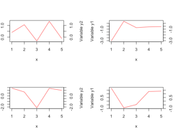
If you need to have two y-axes, the solution is to use a combination of axis() and mtext(). For example: x <- 1:5 y1 <- rnorm(5) y2 <- rnorm(5,20) par(mar=c(5,4,4,5)+.1) plot(x,y1,type="l",col="red") par(new=TRUE) plot(x, y2,,type="l",col="blue",xaxt="n",yaxt="n",xlab="",ylab="") axis(4) mtext("y2",side=4,line=3) legend("topleft",col=c("red","blue"),lty=1,legend=c("The variable y1","The variable y2")) But if you want have several plots in the same graphs, using layout() or mfrow(), a problem occurs because the size of the second y-axe is not the same as the size of the first: layout(matrix(1:4, ncol=2)) x <- 1:5 y1 <- rnorm(5) par(mar=c(5,4,4,5)+.1) plot(x,y1,type="l",col="red", ylab="Variable y1") axis(4) mtext("Variable y2",side=4,line=3) The pro

smoothScatter() plots irregular 2D data with level of colors. However it does not show the z-scale. Here is a way to plot a z-scale: library(graphics) library(fields) n <- 10000 x  <- matrix(rnorm(n), ncol = 2) y  <- matrix(rnorm(n, mean = 3, sd = 1.5), ncol = 2) # dans x, les coordonnées x # dans y, les coordonnées y par(mar=c(4, 4, 2, 6)+0.4) smoothScatter(x, y) n <- matrix(0, ncol=128, nrow=128) xrange <- range(x) yrange <- range(y) for (i in 1:length(x)) {   posx <- 1+floor(127*(x[i]-xrange[1])/(xrange[2]-xrange[1]))   posy <- 1+floor(127*(y[i]-yrange[1])/(yrange[2]-yrange[1]))   n[posx, posy] <- n[posx, posy]+1 } image.plot( legend.only=TRUE, zlim= c(0, max(n)), nlevel=128, col=colorRampPalette(c("white", blues9))(128))

Whereas it is very simple to inverse the logit function [p=1/(1+exp(x)), x=log((1-p)/p)], I had some difficulties with the probit one. Here is the solution using pnorm(). > data <- data.frame(Doses=c(80, 120, 150, 150, 180, 200), +                    Alive=c(10, 12, 8, 6, 2, 1), +                    Dead=c(0, 1, 5, 6, 9, 15)) > ep <- glm(cbind(Alive, Dead) ~ Doses, data=data, family=binomial(link="probit")) > ep$coefficients (Intercept)       Doses   5.74329978 -0.03690572  > ep$coefficients["(Intercept)"]+ep$coefficients["Doses"]*data$Doses [1]  2.7908421  1.3146132  0.2074416  0.2074416 -0.8997301 -1.6378445 > pnorm(ep$coefficients["(Intercept)"]+ep$coefficients["Doses"]*data$Doses) [1] 0.99737144 0.90568004 0.58216749 0.58216749 0.18413196 0.05072707 > predict(ep)          1          2          3          4          5          6   2.7908421  1.3146132  0.2074416  0.2074416 -0.899

The objective is to merge two named vectors and if some variables have common name, only one is used. It is similar is modifyList() but applied to vector. The trick is to convert vectors as lists, and unlist them at the end to return vectors: unlist(modifyList(as.list(A), as.list(B))) > A <- c(K=1, L=2) > B <- c(X=3, Y=0, Z=2) > # No common name, it makes just a concatenation  > unlist(modifyList(as.list(A), as.list(B))) K L X Y Z  1 2 3 0 2  > A <- c(K=1, L=2, X=10) > # X is common, only the second one is used > unlist(modifyList(as.list(A), as.list(B))) K L X Y Z  1 2 3 0 2  > B <- NULL > # If one is NULL, just return the first one > unlist(modifyList(as.list(A), as.list(B))) K  L  X  1  2 10  > B <- c(X=3, Y=0, Z=2) > A <- NULL > unlist(modifyList(as.list(A), as.list(B))) X Y Z  3 0 2 This trick has been introduced as a function modifyVector() in the packages HelpersMG():

The best practice is to use list(...) to read the parameters transmitted through ... It will return a list. Examples: > es <- function(...) {str(list(...))} > es() list() > es(1) List of 1 $ : num 1 > es(c(1, 2)) List of 1 $ : num [1:2] 1 2 > es(r=3, c(1, 2)) List of 2 $ r: num 3 $  : num [1:2] 1 2 > es(las=1, xlim=c(1,2)) List of 2 $ las : num 1 $ xlim: num [1:2] 1 2 If you want read the ... both within a function and in interactive mode for example for debugging: troispoints <- tryCatch(list(...), error=function(e) list())