Articles

Affichage des articles du juillet, 2017

rJava package in r-devel 3.5

rJava package used /usr/local/clang4 folder to search bin/clang compiler. However clang4 is relatively old now. We will use most recent version of clang: brew install llvm clang 5.0.1 (at the time of writing this note) will be install in: /usr/local/opt/llvm/bin/clang Then, do: cd /usr/local sudo ln -s /usr/local/opt/llvm clang4 However, it fails to find the libomp Do: sudo ln -s /Library/Frameworks/R.framework/Versions/3.5/Resources/lib/libomp.dylib libomp.dylib Now you can do in R: install.packages("rJava") Still two problems to solve: - do not setup JAVA_HOME in your .profile or it will make an error when you load the library - If you use Rstudio, you must enter these commands due to a bug in Rstudio cd /usr/local/lib sudo ln -s /Library/Java/JavaVirtualMachines/jdk1.8.0_162.jdk/Contents/Home/jre/lib/server/libjsig.dylib libjsig.dylib sudo ln -s /Library/Java/JavaVirtualMachines/jdk1.8.0_162.jdk/Contents/Home/jre/lib/server/libjvm.dylib libjvm.dy

gfortran 6.3.0 to compile package

Update: 30/7/2021 The latest gfortran is package in gcc for Mac brew: First install homebrew, using in terminal: /usr/bin/ruby -e "$(curl -fsSL https://raw.githubusercontent.com/Homebrew/install/master/install)" Then install llvm brew install --with-clang llvm The latest version of fortran can be found here: https://gcc.gnu.org/wiki/GFortranBinaries#MacOS It is currently the version 6.3.0 for Sierra. However some packages still want use the 6.1.0 version for installation. Here is a solution to update gfortran. First, remove all previous old fortran installation, for example the 4.8.2: Here is the code from http://thecoatlessprofessor.com/programming/rcpp-rcpparmadillo-and-os-x-mavericks-lgfortran-and-lquadmath-error/ # Download installer into working directory curl -O http://r.research.att.com/libs/gfortran-4.8.2-darwin13.tar.bz2 # Remove _files_ associated with the binary for file in $( tar tfz gfortran-4.8.2-darwin13.tar.bz2 ) ; do sudo rm -f / $file ; done

IP adresses on MacosX, Ubuntu or windows

x <- system("ifconfig", intern=TRUE); gsub("^(.*)[ :]([0-9\\.]+) (.*)$", "\\2", x[grep("inet ", x)]) In windows (I cannot test it): x <- system("ipconfig", intern=TRUE); gsub(".*? ([[:digit:]])", "\\1", x[grep("IPv4", x)])

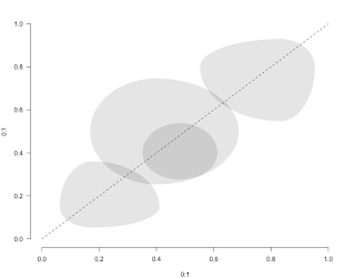
Bivariate confidence interval as a bubble (irregular ellipse)

Image
This function will be useful if you want show the confidence interval of bivariate plots as a bubble (an irregular ellipse). Note that this function has been introduced and enhanced in my package HelpersMG available in CRAN ellipse <- function(center.x = 0, center.y = 0,                         radius.x = 1, radius.y = 1,                         radius.x.lower=NULL, radius.x.upper=NULL,                         radius.y.lower=NULL, radius.y.upper=NULL, col=rgb(0, 0, 0, 0.1)) {   if (is.null(radius.x.lower))  radius.x.lower <- radius.x   if (is.null(radius.y.lower))  radius.y.lower <- radius.y   if (is.null(radius.x.upper))  radius.x.upper <- radius.x   if (is.null(radius.y.upper))  radius.y.upper <- radius.y   for (k in seq_along(center.x)) {   theta <- seq(0, pi / 2, length=100)   x <- center.x[k] + radius.x.upper[k] * cos(theta)   y <- center.y[k] + radius.y.upper[k] * sin(theta)   theta <- seq(pi / 2, pi, length=100)   x <- c(x, cente

Custom axis for image.plot() from fields package

It was a bug in R that has been corrected in r-devel (r72982). Thanks to Paul Murrell <paul@stat.auckland.ac.nz> ______________________________________ For an obscur reason, it is not possible to customize axes of the "big plot" done with image.plot() from package fields: library(fields) par(mar=c(5,4.5,4,7)) D <- matrix(c(10, 20, 25, 30, 12, 22, 32, 35, 13, 25, 38, 40), nrow=3) image.plot(D, col=rev(heat.colors(128)),bty="n", xlab="Lines",        ylab="Columns", cex.lab = 0.5, zlim=c(min(D, na.rm=TRUE),max(D, na.rm=TRUE)),        las=1, axes=FALSE) axis(1, at=seq(from=0, to=1, length=nrow(D)), labels=0:2, cex.axis=0.5) axis(2, at=seq(from=0, to=1, length=ncol(D)), labels=0:3, las=1, cex.axis=0.5) First solution: plot separately the heatmap and the legend: image(D, col=rev(heat.colors(128)),bty="n", xlab="Lines",        ylab="Columns", cex.lab = 0.5, zlim=c(min(D, na.rm=TRUE),max(D, na.rm=T