Zero-truncated negative binomial distribution

First, let try a NB distribution with mu and theta:
mu <- 3; theta <- 2.4

d <- NULL; for (i in 0:20) d <- c(d, dnbinom(i, size=theta, mu=3, log=FALSE))
sum(d)
The sum of probability mass functions is 1. All is perfect.

Let do a zero-truncated negative binomial distribution after Girondot M (2010) Editorial: The zero counts. Marine Turtle Newsletter 129: 5-6 

e <- d[-1]/(1-d[1])
sum(e)
The sum of probability mass functions is 1. All is perfect again.

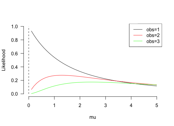
Let estimate the likelihood of observations when mu varies. The idea is to check what mu value will be selected using optim()
obs <- 1
f <- NULL
s <- seq(from=0, to=5, by=0.1)
for (mu in s)
  f <- c(f , dnbinom(obs, size=theta, mu=mu, log=FALSE)/(1-dnbinom(0, size=theta, mu=mu, log=FALSE)))
plot(s, f, type="l", bty="n", las=1, ylim=c(0, 1), xlab="mu", ylab="Likelihood")

obs <- 2
f <- NULL
s <- seq(from=0, to=5, by=0.1)
for (mu in s)
  f <- c(f , dnbinom(obs, size=theta, mu=mu, log=FALSE)/(1-dnbinom(0, size=theta, mu=mu, log=FALSE)))
lines(s, f, col="red")

obs <- 3
f <- NULL
s <- seq(from=0, to=5, by=0.1)
for (mu in s)
  f <- c(f , dnbinom(obs, size=theta, mu=mu, log=FALSE)/(1-dnbinom(0, size=theta, mu=mu, log=FALSE)))
lines(s, f, col="green")

segments(x0=0, x1=0, y0=0, y1=1, lty=2)
legend("topright", legend=c("obs=1", "obs=2", "obs=3"), col=c("black", "red", "green"), lty=1)

For 1 observation, the fitted mu is limit(mu ->0) but excluding mu = 0 because it is not defined.

# dnbinom is the probability mass function

k <- 1
m <- 3
r <- 2.4

First test how dnbinom() is parametrized:
(gamma(r+k)/(factorial(k)*gamma(r)))*(r/(r+m))^r*(m/(r+m))^k
dnbinom(k, size=theta, mu=mu, log=FALSE)

Second test how two solutions of zero-truncated negative binomial is parametrized:
After Arrabal CT, dos Santos Silva KP, Bandeira LN (2014) Zero-truncated negative binomial applied to nonlinear data. JP Journal of Biostatistics 11: 55-67
(gamma(r+k)/(factorial(k)*gamma(r)))*(r/(r+m))^r*(m/(r+m))^k*(1-((r/(r+m))^r))^-1
After Girondot M (2010) Editorial: The zero counts. Marine Turtle Newsletter 129: 5-6
dnbinom(k, size=theta, mu=mu, log=FALSE)/(1-dnbinom(0, size=theta, mu=mu, log=FALSE))

Both are identical.

But note that calling a function is slower than doing inline calculation.

> dnbinom_bis <- function(x, size, mu) {
+   (gamma(size+x)/(factorial(x)*gamma(size)))*(size/(size+mu))^size*(mu/(size+mu))^x
+ }
> system.time({for (i in 1:100000) dnbinom(k, size=r, mu=m, log=FALSE)})
utilisateur     système      écoulé
      0.173       0.001       0.176
> system.time({for (i in 1:100000) dnbinom_bis(k, size=r, mu=m)})
utilisateur     système      écoulé
      0.185       0.003       0.188
> system.time({for (i in 1:100000) (gamma(r+k)/(factorial(k)*gamma(r)))*(r/(r+m))^r*(m/(r+m))^k})
utilisateur     système      écoulé
      0.085       0.000       0.085

On the other hand, for very high size or mu, dnbinom() can report the value whereas inline calculation produced an error.