Articles

Affichage des articles du 2018

SE for all levels of a factor after a glmm

When you are doing a LM, GLM or GLMM with fixed effect with categorical variable, it is impossible to get the SE for all levels because always one level is fixed to 0. But sometimes, you need to know how this level is really known. Two solutions are presented for this problem. The first solution is to force the intercept to be 0 but it works only when there is only one categorical fixed factor. The second is to use a method know as quasi-variance: Firth, D., de Mezezes, R.X., 2004. Quasi-variances. Biometrika 91, 65-80. It is available in package qvcalc for lm() and glm() and in package HelpersMG for lmer(). Here is an example with lmer(): x <- rnorm(100) y <- rnorm(100) G <- as.factor(sample(c("A", "B", "C", "D"), 100, replace = TRUE)) H <- as.factor(sample(c("A", "B", "C", "D"), 100, replace = TRUE)) R <- as.factor(rep(1:25, 4)) G <- relevel(G, "A") H <-

Insert a plot as a vignette in another plot

Image
Let show how to use par(fig=c(x0, x1, y0, y1)) library(maps) par(fig=c(0, 1, 0, 1)) par(mar=c(4, 4, 1, 2)) map("world", region=c("Sao Tome and Principe:Ilha da Sao Tome",                       "Sao Tome and Principe:Ilha do Principe"),     xlim=c(6, 8), ylim=c(0,2),     asp=1) library(sp) degAxis(side=1, cex.axis=0.8) # in package sp degAxis(side= 2, las=1, cex.axis=0.8) par(fig=c(0.5, 0.9, 0.1, 0.5)) par(new=TRUE) par(mar=c(0, 0, 0, 0)) plot(x=c(-180,180), y=c(-90,90), type="n", axes=FALSE, xlab="n", ylab="n") polygon(x=c(-180, -180, 180, 180), y=c(-90, 90, 90, -90)) par(new=TRUE) map("world", asp=1, add=TRUE, fill=TRUE, col="grey", border=NA) polygon(x=c(6, 6, 8, 8), y=c(0, 2, 2, 0)) library(maps) par(fig=c(0, 1, 0, 1)) par(mar=c(4, 4, 1, 2)) map("world", region=c("Sao Tome and Principe:Ilha da Sao Tome",                       "Sao Tome and Pr

What to do with error : ERROR: failed to lock directory ‘/usr/local/lib/R/site-library’ for modifying

Just after this advice appears: Try removing ‘/usr/local/lib/R/site-library/00LOCK-quantreg’ Then I did: cd /usr/local/lib/R/site-library/ sudo rm -rf 00LOCK-quantreg And I could install the package

Install rJava on ubuntu 18.04

sudo apt-get install openjdk-11-jdk sudo R CMD javareconf JAVA_HOME= /usr/lib/jvm/java-11-openjdk-amd64 sudo R install.packages("rJava")

A parallelized version of for loop

# A general procedure for parallelized for loop # Even with 4 cores, the gain is interesting # Let take this example A <- 1:10000 system.time({ out <- NULL for (i in A) {   # I do something with i, an element of A   # this part must be copied   j <- sqrt(i)   out <- c(out, j)   # I go out of the loop } }) library("parallel") system.time({ B <- split(A, cut(A, detectCores(), labels = FALSE)) out <- unname(unlist(mclapply(B, FUN= function(Bi) {   outi <- NULL   for (i in Bi) {     # I do something with i, an element of A     j <- sqrt(i)     outi <- c(outi, j)     # I go out of the loop   }   return(outi) }))) })

Analyse de la sensibilité de la sortie d'un automate cellulaire

Image
Analyse de la sensibilité d'un automate cellulaire # Fonction qui calcule le nombre de cases occupées (=1) en fonction d'une variable X # qui est un data.frame qui contient les probabilités de mourir à chaque pas de temps (p) et  # le nombre de cases (/9) pour obtenir un décès d'étouffement. # La variable t donne les temps pour lesquels on retourne la taille de la population # Si t est une valeur, on retourne juste la valeur pour ce temps, si t est un vecteur,  # on retourne toutes les valeurs pour les temps t ac <- function(X, t=t) {   Nfinal <- NULL   for (grandtotal in 1:nrow(X)) {     penc <- X[grandtotal, 1]     v <- X[grandtotal, 2]*9     m <- matrix(data = 0, ncol=12, nrow=12)   for (i in 1:10) {     col <- sample(1:10, 1)+1     row <- sample(1:10, 1)+1     m[row, col] <- 1   }   N <- NULL   for (tps in 1:max(t)) {     m1 <- m       for (col in 2:11) {       for (row in 2:11) {         voisins <- sum(

The mess of linear regressions

Image
Everyone has done a linear regression... but not everyone knows really how to do a linear regression. There are several methods which produce different outputs. Here is a little synthesis: # Let generate data. Note the the scale for x and y are different. # the set.seed(1) makes sure that the data are always the same # to make reproduced examples set.seed(1) x <- 1:10 y <- 10*x+rnorm(10, 5, 20) plot(x, y, bty="n", las=1) # First method. Only error on y axis is supposed # The square of the residuals on y axis is minimized # Why the sum of square? It is grounded on the likelihood of Gaussian distribution for residuals lm(y~ x) abline(lm(y~ x), col="red") # second, very similar to previous one, only error on x axis is supposed # The square of the residuals on x axis is minimized ir <- coef(lm(x~y)) print(c(-ir[1]/ir[2],1/ir[2])) abline(-ir[1]/ir[2],1/ir[2], col="blue") # The choice between error inputed

To read grib and grib2 file format

grib and grib2 are format used to store meteorological data. It is the native format used by ECMWF server. To read it in R with MacOSX: Using Macport, install the library wgrib2: sudo port install wgrib2 You must also install the wgrib library: Look at here: https://rda.ucar.edu/datasets/ds083.2/software/wgrib_install_guide.txt Then you can install rNOMAD package in R You must install gdal library You can use also the raster package with rgdal and goal library 4 packages can be used: rNOMAD, rgdal, raster, stars I found that the simple is to use rgdal

Migration to MacOSX 10.14 Mojave

After install, open Xcode and install commande line tools at front. In terminal: sudo xcodebuild -license type agree after many pages then sudo xcode-select --install defaults write org.R-project.R force.LANG fr_FR.UTF-8 sudo installer -pkg /Library/Developer/CommandLineTools/Packages/macOS_SDK_headers_for_macOS_10.14.pkg -target /

Bayesian or frequentist test

This note is based on a discussion with Jean-Michel Guillon. The idea was to test an idea from this this paper: Sterne, J.A.C., Smith, G.D., 2001. Sifting the evidence-what’s wrong with significance tests? British Medical Journal 322, 226-231. If our prior opinion about the risk ratio is vague (we consider a wide range of values to be equally likely) then the results of a frequentist analysis are similar to the results of a bayesian analysis; both are based on what statisticians call the likelihood for the data: • The 95% confidence interval is the same as the 95% credible interval, except that the latter has the meaning often incorrectly ascribed to a confidence interval; • The (one sided) P value is the same as the bayesian posterior probability that the drug increases the risk of death (assuming that we found a protective effect of the drug). The two approaches, however, will give different results if our prior opinion is not vague, relative to the amount of informatio

On the use of OR | operator in regular expression

I had some difficulties to use the OR | operator in regular expressions. Let do some exercises and examine the results: gregexpr("bc", "abcd") : return 2; normal, bc is located at the second position gregexpr("b|c", "abcd") : return 2 3; | is the OR operator and it will return the position of b OR c this is the same than : gregexpr("[bc]", "abcd") or gregexpr("[b|c]", "abcd") But | and [] are not always the same: Let do more complicated: gregexpr("ab|cd", "abcd") My problem was about the priority order of | operator. The return here is 1 3 It means that the search was for a followed by b OR c followed by d. Let do more complicated : gregexpr("a[bc]d", "abcd") : return -1; it search for abd or acd. None exist In practice, it is good to remember that | separates blocks of comparisons.

[0-9] or \d or [:digit:] in grep

If you want search for a number using grep, you have 4 options: [0123456789] or [0-9] or \d or [:digit:] Here is a comparison: library(microbenchmark) microbenchmark({grep(pattern="[0123456789][0123456789][0123456789][0123456789]", "Ussiosuus8980JJDUD98")},                 {grep(pattern="[0-9][0-9][0-9][0-9]", "Ussiosuus8980JJDUD98")},                 {grep(pattern="[[:digit:]][[:digit:]][[:digit:]][[:digit:]]", "Ussiosuus8980JJDUD98")},                 {grep(pattern="\\d\\d\\d\\d", "Ussiosuus8980JJDUD98")}, times = 1000L)     min      lq      mean  median      uq    max neval  cld  21.729 22.1840 22.887585 22.3090 22.4645 64.542  1000    d   5.219  5.3740  5.696937  5.4665  5.8495 47.618  1000 a       9.778 10.0425 10.482301 10.1470 10.5400 25.602  1000  b    10.296 10.5000 11.099359 10.6360 11.0440 39.759  1000   c  Clearly the solution [0-9] is the best This is the same for l

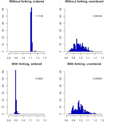
Forking or not for parallel computing

Image
In linux, forking is available when parallel computing is done but not in Windows. But what is the difference ? Let do an exemple (code is below): When the durations of the tasks are unordered, both algorithms are performing identically. However when task durations are ordered, forking is doing much better. library(parallel) l <- (1:32)/10/16.5 sum(l) t0 <- system.time(lapply(l, FUN=function(x) {Sys.sleep(x)}))["elapsed"] cl <- makeCluster(detectCores()) out1 <- NULL; for (i in 1:200) out1 <- c(out1, system.time(parLapplyLB(cl = cl, X = l, fun = function(x) {Sys.sleep(x)}))["elapsed"]) stopCluster(cl) out2 <- NULL; for (i in 1:200) out2 <- c(out2, system.time(mclapply(l, mc.cores =detectCores(), FUN=function(x) {Sys.sleep(x)}))["elapsed"]) cl <- makeCluster(detectCores()) out3 <- NULL; for (i in 1:200) out3 <- c(out3, system.time(parLapplyLB(cl = cl, X = l[sample(32)], fun = function(x) {Sys.sleep(x)})

Performance of grepl versus more crude method using substr() and ==

I wanted test if the name of parameters begins with max. First I used a rather crude substr(var, begin, length) and then I had a better idea: using grepl. But was the more crude version really the worst ? Here is a little test that permits to use the function microbenchmark in the package of the same name. > times <- microbenchmark( grepl("^max", "max_152"), substr("max_152", 1, 3) == "max", times=1e3) > times Unit: nanoseconds expr min lq mean median uq max neval grepl("^max", "max_152") 3980 4255 4863.691 4539.5 4941.0 30161 1000 substr("max_152", 1, 3) == "max" 995 1205 1492.998 1340.5 1579.5 16659 1000 The returned data frame has the following informations: expr: the tested expressions neval: how many time they have been evaluated min, lq, mean, median, uq, max are respectively the minimum, lower quartile, mean, median, upper quar

On the error bar and statistical significance

Image
Take two random series of 20 values. What you can tell about their difference according to the visualization of their confidence interval: nearly nothing ! Let use this little script: library(HelpersMG) x <- rnorm(20, mean=11.8, sd=2) y <- rnorm(20, mean=10, sd=2) t <- t.test(x, y, var.equal = TRUE) w <- series.compare(x, y, criterion = c("BIC"), var.equal = TRUE) plot_errbar(x=1:2, y=c(mean(x), mean(y)), errbar.y=1.96*c(sd(x), sd(y)),             las=1, bty="n", xlab="", ylab="", ylim=c(0, 20), xlim=c(0, 3)) plot_errbar(x=(1:2)+0.1, y=c(mean(x), mean(y)), errbar.y=2*c(sd(x)/sqrt(20), sd(y)/sqrt(20)),             las=1, bty="n", xlab="", ylab="", ylim=c(0, 20), xlim=c(0, 3), add=TRUE, col="red",             errbar.col = "red") text(x = 1.5, y=2, labels = paste0("p = ", format(t$p.value, digits = 5))) text(x = 1.5, y=3, labels = paste0("w = ", forma

Error during packages compilation about -lomp

If you have an error about -lomp, y ou must verify that you have libomp.dylib. The simplest way to do is to in terminal and  activate locate database: sudo /usr/libexec/locate.updatedb This function can be used also to update the database. Then you can do: locate libomp.dylib  | xargs ls -l And the result is for example: -rwxrwxr-x  1 root          admin  508044 26 aoû 22:31 /Library/Frameworks/R.framework/Versions/3.5/Resources/lib/libomp.dylib -r--r--r--  1 marcgirondot  admin  442396 31 jan  2018 /usr/local/Cellar/llvm/5.0.1/lib/libomp.dylib -r--r--r--  1 marcgirondot  admin  491820 12 mar 09:38 /usr/local/Cellar/llvm/6.0.0/lib/libomp.dylib -r--r--r--  1 marcgirondot  admin  495888  6 jul 17:11 /usr/local/Cellar/llvm/6.0.1/lib/libomp.dylib Choose the one that you want (here the first one because it is the most recent), and do: sudo ln -s /Library/Frameworks/R.framework/Versions/3.5/Resources/lib/libomp.dylib /usr/local/lib/libomp.dylib

Development version of optimx

optimx is a nice replacement of  optim(): install.packages("optimx", repos="http://R-Forge.R-project.org") See  optimx for R - Journal of Statistical Software

Update a package and the dependencies

update.packages(checkBuilt=TRUE, ask=FALSE)

Install rJava in R 3.6 with MacOSX 10.13

Instal homebrew:  https://brew.sh/index_fr In terminal: brew install --with-toolchain llvm in .profile, add: PATH="/usr/local/opt/llvm/bin:${PATH}" LDFLAGS="-L/usr/local/opt/llvm/lib -Wl,-rpath,/usr/local/opt/llvm/lib" CPPFLAGS="-I/usr/local/opt/llvm/include" export LDFLAGS export CPPFLAGS Install the latest java jdk:  http://www.oracle.com/technetwork/java/javase/downloads/jdk8-downloads-2133151.html Look at here:  https://biostatsr.blogspot.fr/2018/02/set-javahome-to-correct-value-in-profile.html In terminal, enter: cd $(/usr/libexec/java_home)/jre/bin/ sudo ln  $(/usr/libexec/java_home) /bin/javac javac sudo ln  $(/usr/libexec/java_home) /bin/javah javah sudo ln  $(/usr/libexec/java_home) /bin/jar jar cd  $(/usr/libexec/java_home)/jre/lib/ sudo ln  $(/usr/libexec/java_home) /lib/tools.jar tools.jar cd $HOME sudo R CMD javareconf And in R install.packages("rJava")