BiostatR Blog

The prior for proportion should be chosen within Beta distribution.  Beta distribution in Wikipedia Beta distribution has two parameters, alpha and beta (alpha>0 and beta>0) and it used a parameter 0≤x≤1. x can be a proportion. For such a reason, Beta distribution is perfect to be used as a prior for proportion. Look at the shape of beta: colors = c("red","blue","green","orange","purple", "black") grid = seq(0,1,.01) alpha = c(.5,5,1,2,2, 1) beta = c(.5,1,3,2,5, 1) plot(grid,grid,type="n",xlim=c(0,1),ylim=c(0,4),xlab="",ylab="Prior Density",      main="Prior Distributions", las=1) for(i in 1:length(alpha)){   prior = dbeta(grid,alpha[i],beta[i])   lines(grid,prior,col=colors[i],lwd=2) } legend("topleft", legend=c("Beta(0.5,0.5)", "Beta(5,1)", "Beta(1,3)", "Beta(2,2)", "Beta(2,5)", "Beta(1,1)"),...

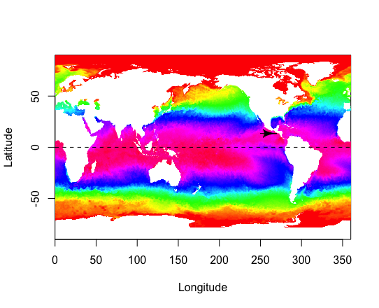
library("HelpersMG") # Guatemala map # get the ncdf file here for 2010, 2011, 2012 # <a href="http://www.esrl.noaa.gov/psd/cgi-bin/db_search/DBListFiles.pl?did=132&tid=33865&vid=2423">http://www.esrl.noaa.gov/psd/cgi-bin/db_search/DBListFiles.pl?did=132&tid=33865&vid=2423</a> # ftp://ftp.cdc.noaa.gov/Datasets/noaa.oisst.v2.highres/sst.day.mean.2012.v2.nc # ftp://ftp.cdc.noaa.gov/Datasets/noaa.oisst.v2.highres/sst.day.mean.2011.v2.nc # ftp://ftp.cdc.noaa.gov/Datasets/noaa.oisst.v2.highres/sst.day.mean.2010.v2.nc url <- "ftp://ftp.cdc.noaa.gov/Datasets/noaa.oisst.v2.highres/sst.day.mean.2012.v2.nc" dest <- paste(Sys.getenv("HOME"), "/sst.day.mean.2012.v2.nc", sep="") download.file(url, dest) url <- "ftp://ftp.cdc.noaa.gov/Datasets/noaa.oisst.v2.highres/sst.day.mean.2011.v2.nc" dest <- paste(Sys.getenv("HOME"), "/sst.day.mean.2011.v2.nc",...

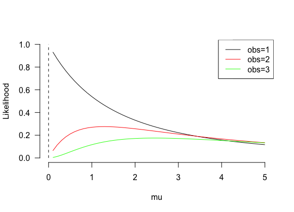
First, let try a NB distribution with mu and theta: mu <- 3; theta <- 2.4 d <- NULL; for (i in 0:20) d <- c(d, dnbinom(i, size=theta, mu=3, log=FALSE)) sum(d) The sum of probability mass functions is 1. All is perfect. Let do a zero-truncated negative binomial distribution after Girondot M (2010) Editorial: The zero counts. Marine Turtle Newsletter 129: 5-6  e <- d[-1]/(1-d[1]) sum(e) The sum of probability mass functions is 1. All is perfect again. Let estimate the likelihood of observations when mu varies. The idea is to check what mu value will be selected using optim() obs <- 1 f <- NULL s <- seq(from=0, to=5, by=0.1) for (mu in s)   f <- c(f , dnbinom(obs, size=theta, mu=mu, log=FALSE)/(1-dnbinom(0, size=theta, mu=mu, log=FALSE))) plot(s, f, type="l", bty="n", las=1, ylim=c(0, 1), xlab="mu", ylab="Likelihood") obs <- 2 f <- NULL s <- seq(from=0, to=5, by=0.1) for (mu in s)   f <...

Let do: > as.character(as.Date("2020-06-07"), format="%d/%m/%y") [1] "07/06/20" But what to do if you want just 7/6/20 ? Here is the solution: > gsub("^0", "", gsub("([-])0", "\\1", as.character(as.Date("2020-06-07"), format="%d/%m/%y"))) [1] "7/06/20" Or > d <- as.character(as.Date("2020-06-07"), format="%d/%m/%y") > gsub("^0", "", gsub("/0", "/", d)) [1] "7/6/20"