BiostatR Blog

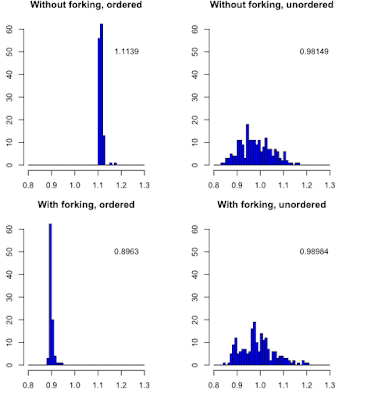
In linux, forking is available when parallel computing is done but not in Windows. But what is the difference ? Let do an exemple (code is below): When the durations of the tasks are unordered, both algorithms are performing identically. However when task durations are ordered, forking is doing much better. library(parallel) l <- (1:32)/10/16.5 sum(l) t0 <- system.time(lapply(l, FUN=function(x) {Sys.sleep(x)}))["elapsed"] cl <- makeCluster(detectCores()) out1 <- NULL; for (i in 1:200) out1 <- c(out1, system.time(parLapplyLB(cl = cl, X = l, fun = function(x) {Sys.sleep(x)}))["elapsed"]) stopCluster(cl) out2 <- NULL; for (i in 1:200) out2 <- c(out2, system.time(mclapply(l, mc.cores =detectCores(), FUN=function(x) {Sys.sleep(x)}))["elapsed"]) cl <- makeCluster(detectCores()) out3 <- NULL; for (i in 1:200) out3 <- c(out3, system.time(parLapplyLB(cl = cl, X = l[sample(32)], fun = function(x) {Sys.sleep(x)})

I wanted test if the name of parameters begins with max. First I used a rather crude substr(var, begin, length) and then I had a better idea: using grepl. But was the more crude version really the worst ? Here is a little test that permits to use the function microbenchmark in the package of the same name. > times <- microbenchmark( grepl("^max", "max_152"), substr("max_152", 1, 3) == "max", times=1e3) > times Unit: nanoseconds expr min lq mean median uq max neval grepl("^max", "max_152") 3980 4255 4863.691 4539.5 4941.0 30161 1000 substr("max_152", 1, 3) == "max" 995 1205 1492.998 1340.5 1579.5 16659 1000 The returned data frame has the following informations: expr: the tested expressions neval: how many time they have been evaluated min, lq, mean, median, uq, max are respectively the minimum, lower quartile, mean, median, upper quar

Take two random series of 20 values. What you can tell about their difference according to the visualization of their confidence interval: nearly nothing ! Let use this little script: library(HelpersMG) x <- rnorm(20, mean=11.8, sd=2) y <- rnorm(20, mean=10, sd=2) t <- t.test(x, y, var.equal = TRUE) w <- series.compare(x, y, criterion = c("BIC"), var.equal = TRUE) plot_errbar(x=1:2, y=c(mean(x), mean(y)), errbar.y=1.96*c(sd(x), sd(y)),             las=1, bty="n", xlab="", ylab="", ylim=c(0, 20), xlim=c(0, 3)) plot_errbar(x=(1:2)+0.1, y=c(mean(x), mean(y)), errbar.y=2*c(sd(x)/sqrt(20), sd(y)/sqrt(20)),             las=1, bty="n", xlab="", ylab="", ylim=c(0, 20), xlim=c(0, 3), add=TRUE, col="red",             errbar.col = "red") text(x = 1.5, y=2, labels = paste0("p = ", format(t$p.value, digits = 5))) text(x = 1.5, y=3, labels = paste0("w = ", forma