Runge-Kutta algorithm

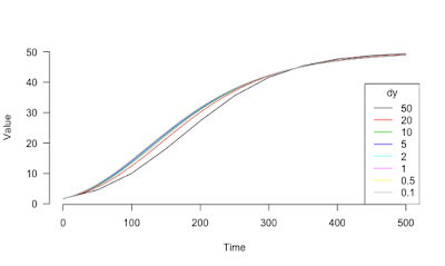
Test of the Runge-Kutta algorithm and comparison with implementation within the deSolve package or the approximation dy -> 0.
The code for Runge-Kutta algorithm has been done by Maxime Jacquemin (ESE, University Paris Sud). It does a little bit better that the deSolve code but very little.

> # from package embryogrowth
> # function lsoda wants a list
> dydt.Gompertz <- function(t, size, parms) {
+   dy.dt <- parms["alpha"]*log(parms["K"]/size)*size
+   list(dy.dt)
+ }
> 
> # Same function but returns a vector
> dydt.Gompertz_2 <- function(t, size, parms) {
+   dy.dt <- parms["alpha"]*log(parms["K"]/size)*size
+   dy.dt
+ }
> 
> # Integration of Gompertz function
> Gompertz <- function(x, y0, K, alpha) {
+   return(K*exp(log(y0/K)*exp(-alpha*x)))
+ }
> 
> # Fonction d'intégration numérique par la méthode de Runge-Kutta
> # par Maxime Jacquemin
> Runge.Kutta <- function(y, times, func, parms = NULL)
+ {
+   n.iter <- length(times)
+   results <- rep(y, n.iter)
+   yn <- y
+ 
+   for (i in 2:n.iter)
+   {
+     h <- times[i] - times[i-1]
+     tn <- times[i - 1]
+     k1 <- func(tn, yn, parms)
+     k2 <- func(tn + (h / 2), yn + (h / 2) * k1, parms)
+     k3 <- func(tn + (h / 2), yn + (h / 2) * k2, parms)
+     k4 <- func(tn + h, yn + h * k3, parms)
+     yn <- yn + (h / 6) * (k1 + 2 * k2 + 2 * k3 + k4)
+     results[i] <- yn
+   }
+   
+   return(data.frame(times, results))
+ }
> 
> xv <- seq(from=0, to =500, by=10)
> yv <- Gompertz(xv, y0=1.7, K=50, alpha=0.01)
> 
> plot(x = xv, 
+      y = yv, 
+      type="l", bty="n", xlab="Time", ylab="Value", las=1)
> df <- data.frame(time=xv[1:6], Gompertz=yv[1:6])
> 
> # using the approximation dy/dx when dx -> 0
> index <- 1
> for (dy in c(50, 20, 10, 5, 2, 1, 0.5, 0.1)) {
+ x <- seq(from=0, to =500, by=dy)
+ y <- rep(1.7, length(x))
+ for (i in 2:length(x))
+   y[i] <- y[i-1] + dydt.Gompertz_2(x[i], y[i-1], parms=c(K=50, alpha=0.01))*dy
+ dfi <- as.data.frame(list(y[match(xv[1:6], x)]), col.names=paste0("dy.", as.character(dy)))
+ df <- cbind(df, dfi)
+ lines(x, y, col=index)
+ index <- index + 1
+ # text(501, tail(y, 1)+1, as.character(dy), pos=4, xpd=TRUE)
+ }
> 
> legend("bottomright", legend=as.character(c(50, 20, 10, 5, 2, 1, 0.5, 0.1)), 
+        col=1:8, lty=1, title="dy")

> 
> plot(x = xv, 
+      y = yv, 
+      type="l", bty="n", xlab="Time", ylab="Value", las=1)
> 
> dy <- 10
> x <- seq(from=0, to =500, by=dy)
> rk4 <- Runge.Kutta(func = dydt.Gompertz_2, 
+                    times=x, 
+                    y=1.7, 
+                    parms=c(K=50, alpha=0.01)
+                    )
> dfi <- as.data.frame(
+   list(
+     rk4[
+       match(xv[1:6], x)
+       , 2]
+     ), col.names="rk4")
> df <- cbind(df, dfi)
> 
> 
> system.time(for (i in 1:10000) 
+   Runge.Kutta(func = dydt.Gompertz_2, 
+               times=x, 
+               y=1.7, 
+               parms=c(K=50, alpha=0.01)
+               )
+   )
utilisateur     système      écoulé 
     19.460       0.197      19.766 
> points(rk4[, 1], rk4[, 2], pch=1)
> 
> 
> library(deSolve)
> dy <- 10
> x <- seq(from=0, to =500, by=dy)
> rk4_desolve <- lsoda(func = dydt.Gompertz, 
+                      times=x, 
+                      y=1.7, 
+                      parms=c(K=50, alpha=0.01))
> dfi <- as.data.frame(list(rk4_desolve[match(xv[1:6], x), 2]), col.names="rk4.deSolve")
> df <- cbind(df, dfi)
> 
> system.time(for (i in 1:10000) 
+   lsoda(func = dydt.Gompertz, 
+         times=x, 
+         y=1.7,
+         parms=c(K=50, alpha=0.01)))
utilisateur     système      écoulé 
     19.584       0.187      19.873 
> points(x = rk4_desolve[, 1], rk4_desolve[, 2], pch=4)
> 
> legend("bottomright", 
+        legend=c("Gompertz", 
+                 "Runge-Kutta by M. Jacquemin", 
+                 "lsoda from deSolve package"), 
+        lty=c(1, 0, 0), 
+        pch=c(NA, 1, 4))
> 
> df
  time Gompertz    dy.50    dy.20    dy.10     dy.5     dy.2     dy.1   dy.0.5   dy.0.1
1    0 1.700000 1.700000 1.700000 1.700000 1.700000 1.700000 1.700000 1.700000 1.700000
2   10 2.345293       NA       NA 2.274837 2.307908 2.329776 2.337436 2.341340 2.344499
3   20 3.137954       NA 2.849674 2.977788 3.053283 3.102904 3.120225 3.129038 3.136163
4   30 4.083785       NA       NA 3.817775 3.943819 4.026034 4.054608 4.069120 4.080839
5   40 5.183115       NA 4.482434 4.799842 4.982534 5.100656 5.141509 5.162217 5.178921
6   50 6.430829 4.574186       NA 5.924656 6.167470 6.322978 6.376483 6.403551 6.425356
       rk4 rk4.deSolve
1 1.700000    1.700000
2 2.345268    2.345291
3 3.137904    3.137951
4 4.083711    4.083781
5 5.183020    5.183114
6 6.430713    6.430834