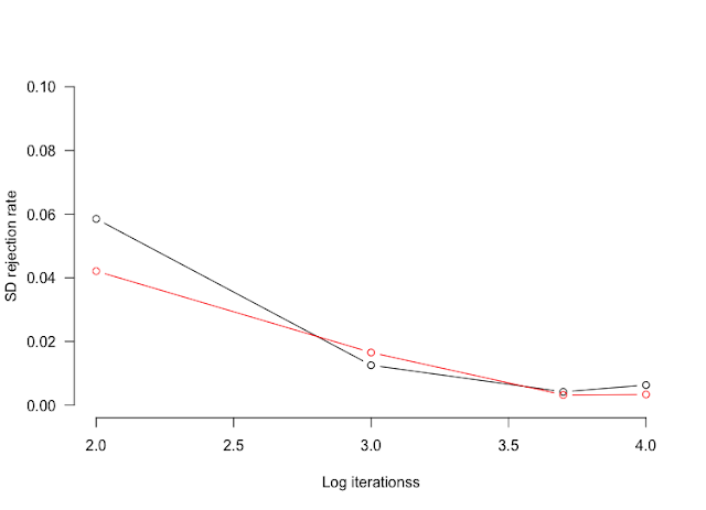
Rejection rate in Metropolis-Hastings algorithm
During the Metropolis-Hastings algorithm run, the rejection rate should be 0.234.
Bédard M. (2008) Optimal acceptance rates for metropolis algorithms: Moving beyond 0.234. Stochastic Processes and Their Applications, 118(12), 2198-2222.
Such a value can be achieved by change of SD proposition parameter for each prior. However it can can tedious to estimate the correct value if each run takes a long time to finish.
However, to get correct rejection rate needs much less iterations than to get correct SD values. Here I will show that with as few as 1000 iterations (10^3), it is possible to estimate rejection rate with a 95% confidence interval at ±0.04.
library(HelpersMG)
# 30 random numbers from Gaussian distribution
x <- rnorm(30, 10, 2)
# Likelihood function
dnormx <- function(data, x) {
data <- unlist(data)
return(-sum(dnorm(data, mean=x['mean'], sd=x['sd'], log=TRUE)))
}
# Where all the results will be stored
RR <- list()
for (iter in c(100, 1000, 5000, 10000)) {
print(iter)
df <- data.frame(mean=as.numeric(), sd=as.numeric())
for (i in 1:10) {
mcmc_run <- MHalgoGen(n.iter=iter, parameters=parameters_mcmc, data=x,
likelihood=dnormx, n.chains=1, n.adapt=100, thin=1, trace=1)
df <- rbind(df, t(as.data.frame(rejectionRate(as.mcmc(mcmc_run)))))
}
RR <- c(RR, list(df))
}
result <- sapply(RR, function(X) apply(X, MARGIN=2, FUN=sd))
plot(log10(c(100, 1000, 5000, 10000)), result["mean", ], bty="n", type="b", las=1,
xlab="Log iterationss", ylab="SD rejection rate", ylim=c(0, 0.1))
plot_add(log10(c(100, 1000, 5000, 10000)), result["sd", ], type="b", col="red")

Commentaires
Enregistrer un commentaire