BiostatR Blog

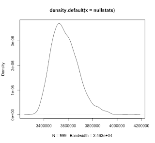
If you want superimpose the theoretical numbers at the top of an histogram based on a fitted distribution (for example, using fitdistrplus()), it is not so easy. Here is a generic function for such a purpose. It is integrated in my package HelpersMG : modeled.hist <- function(breaks, FUN, ..., sum=1) {   # breaks is a vector with the breaks; it can be obtained directly from hist()   # FUN is the function to integrate the density, ex. pnorm   # ... are the parameters of pfun   # sum is the total numbers in the histogram; 1 for emperical frequencies   by <- breaks[2]-breaks[1]   xp <- c(breaks, tail(breaks, 1)+by)   par.fun <- list(...)   par.fun <- modifyList(list(log.p=FALSE, q=xp, lower.tail=TRUE),                          par.fun)   s <- do.call(FUN, par.fun)   # s <- pfun(xp, par.fun[1], par.fun[2], log=FALSE)   s <- head(c(s[-1...

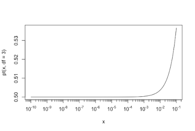
if(!require("sfsmisc")) install.packages("sfsmisc") require("sfsmisc") x <- lseq(1e-10, 0.1, length = 201) plot(x, pt(x, df=3), type = "l", xaxt = "n", log = "x") eaxis(1)

A Mantel test measures the correlation between two matrices typically containing measures of distance.  A Mantel test is one way of testing for spatial autocorrelation. Example of R code: library("vegan") library("fields") library("sp") # Random points points <- as.matrix(data.frame(longitude=rnorm(20, 3, 2), latitude=rnorm(20, 23, 2))) caracteristiques <- rnorm(20, 12, 3) plot(x=points[,"longitude"], y=points[, "latitude"], pch=19, cex=2*caracteristiques/max(caracteristiques)) # matrice des distances euclidiennes de caractéristiques disC <- rdist(x1=caracteristiques) # Matrice de distances entre les points basée sur la distance terrestre disL <- spDists(x=points, longlat = TRUE) plot(disL, disC) MT <- mantel(xdis=disC, ydis=disL, method="pearson", permutations=999) MT

Test of the Runge-Kutta algorithm and comparison with implementation within the deSolve package or the approximation dy -> 0. The code for Runge-Kutta algorithm has been done by Maxime Jacquemin (ESE, University Paris Sud). It does a little bit better that the deSolve code but very little.

A little advantage for seq_along(): l> sibrary(embryogrowth) > system.time(for (i in 1:100000) seq_along(NestsResult)) utilisateur     système      écoulé       0.117       0.012       0.131 > system.time(for (i in 1:100000) 1:length(NestsResult)) utilisateur     système      écoulé       0.143       0.005       0.148

With the help of Julien Nauroy (DI Université Paris Sud) and Maxime Jacquemin (ESE Université Paris Sud) __________________________________________________________________________ To install SparkR, first go there: https://spark.apache.org Download the Spark software choosing these options: - Most recent spark release (1.6.1 at the time of this post written) - Prebuilt for Hadopi 2.6 and later - Direct download You will get a file spark-1.6.1-bin-hadoop2.6.tar in your download folder. Untar it and then you will have a folder: spark-1.6.1-bin-hadoop2.6 Copy this folder in a safe place, for example: ~/Documents/spark-1.6.1-bin-hadoop2.6 ________________________ Two solutions to install the package: library("devtools") Sys.setenv(SPARK_HOME = "~/Documents/spark-1.6.1-bin-hadoop2.6") install(file.path(Sys.getenv("SPARK_HOME"), "R", "lib", "SparkR")) or e nter these commands in R: Sys.setenv(SPARK_HOME = ...

Three different ways to remove first and last elements of a vector are compared. The winner is without contest: v[-c(1, length(v))] > v <- 1:100 > head(v[-1], -1)  [1]  2  3  4  5  6  7  8  9 10 11 12 13 14 15 16 17 18 19 20 21 22 23 24 25 26 27 28 29 30 [30] 31 32 33 34 35 36 37 38 39 40 41 42 43 44 45 46 47 48 49 50 51 52 53 54 55 56 57 58 59 [59] 60 61 62 63 64 65 66 67 68 69 70 71 72 73 74 75 76 77 78 79 80 81 82 83 84 85 86 87 88 [88] 89 90 91 92 93 94 95 96 97 98 99 > rev(rev(v[-1])[-1])  [1]  2  3  4  5  6  7  8  9 10 11 12 13 14 15 16 17 18 19 20 21 22 23 24 25 26 27 28 29 30 [30] 31 32 33 34 35 36 37 38 39 40 41 42 43 44 45 46 47 48 49 50 51 52 53 54 55 56 57 58 59 [59] 60 61 62 63 64 65 66 67 68 69 70 71 72 73 74 75 76 77 78 79 80 81 82 83 84 85 86 87 88 [88] 89 90 91 92 93 94 95 96 97 98 99 > v[-c(1, length(v))]  [1]  2  3  4  5 ...

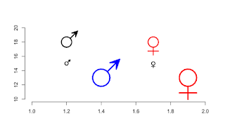
The trick shown here ( http://max2.ese.u-psud.fr/epc/conservation/Girondot/Publications/Blog_r/Entrees/2013/10/22_Males_and_females_symbols.html ) to draw males and females symbols produces ugly symbols. Here are more elegant drawings if you need them in the plot region. These two functions are included in the package HelpersMG. symbol.Male <- function(centerx, centery, rayonx, lwd=2, col="black") { xr <- ScalePreviousPlot()$xlim["range"] yr <- ScalePreviousPlot()$ylim["range"] ratio <- par("pin")[1]/par("pin")[2] rayony <- rayonx*(yr/xr)*ratio angle <- seq(from=0, to=2*pi, length.out = 20) x <- centerx+rayonx*cos(angle) y <- centery+rayony*sin(angle) segments(x0=x, y0=y, x1=x[c(20, 1:19)], y1=y[c(20, 1:19)], col=col, lwd=lwd) x0 = centerx+rayonx*sqrt(2)/2 y0 = centery+rayony*sqrt(2)/2 x1 = centerx+3*rayonx*sqrt(2)/2 y1 = centery+3*rayony*sqrt(2)/2 segments(x0=x0, y0=y0, x1=x1, y1=y1, col=co...

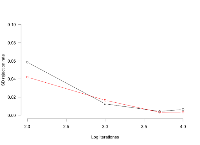
During the Metropolis-Hastings algorithm run, the rejection rate should be 0.234. Bédard M. (2008) Optimal acceptance rates for metropolis algorithms: Moving beyond 0.234. Stochastic Processes and Their Applications, 118(12), 2198-2222. Such a value can be achieved by change of SD proposition parameter for each prior. However it can can tedious to estimate the correct value if each run takes a long time to finish. However, to get correct rejection rate needs much less iterations than to get correct SD values. Here I will show that with as few as 1000 iterations (10^3),  it is possible to estimate rejection rate with a 95% confidence interval at ±0.04. library(HelpersMG) # 30 random numbers from Gaussian distribution  x <- rnorm(30, 10, 2) # Likelihood function dnormx <- function(data, x) {   data <- unlist(data)   return(-sum(dnorm(data, mean=x['mean'], sd=x['sd'], log=TRUE))) } # Where all the results will be stored ...