BiostatR Blog

This article was originally posted in my previous blog Let data that you suppose being distributed as Gaussian distribution. # Generate 100 values from Gaussian distribution val=rnorm(100, mean=20, sd=5) If you want know the mean and sd of the underlying Gaussian distribution, you can use directly mean() and sd() however you will not know the distribution of the mean and SD (ie. if the mean and SD are well known). mean(val); sd(val) To get the distribution of both mean and SD (and then their confidence interval), you can use maximum likelihood and the SE of the point estimates can be obtained from the square root of the inverse of the Hessian matrix. Let do it: # Return -ln L of values in val in Gaussian distribution with mean and sd in par fitnorm<-function(par, val) {   -sum(dnorm(val, par["mean"], par["sd"], log = TRUE)) } # Initial values for search p<-c(mean=20, sd=5) # fit the model result <- optim(par=p, fn=fitnorm, val=val, metho...

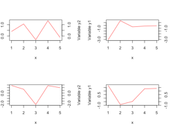
If you need to have two y-axes, the solution is to use a combination of axis() and mtext(). For example: x <- 1:5 y1 <- rnorm(5) y2 <- rnorm(5,20) par(mar=c(5,4,4,5)+.1) plot(x,y1,type="l",col="red") par(new=TRUE) plot(x, y2,,type="l",col="blue",xaxt="n",yaxt="n",xlab="",ylab="") axis(4) mtext("y2",side=4,line=3) legend("topleft",col=c("red","blue"),lty=1,legend=c("The variable y1","The variable y2")) But if you want have several plots in the same graphs, using layout() or mfrow(), a problem occurs because the size of the second y-axe is not the same as the size of the first: layout(matrix(1:4, ncol=2)) x <- 1:5 y1 <- rnorm(5) par(mar=c(5,4,4,5)+.1) plot(x,y1,type="l",col="red", ylab="Variable y1") axis(4) mtext("Variable y2",side=4,line=3) The pro...

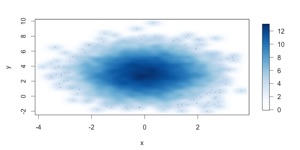
smoothScatter() plots irregular 2D data with level of colors. However it does not show the z-scale. Here is a way to plot a z-scale: library(graphics) library(fields) n <- 10000 x  <- matrix(rnorm(n), ncol = 2) y  <- matrix(rnorm(n, mean = 3, sd = 1.5), ncol = 2) # dans x, les coordonnées x # dans y, les coordonnées y par(mar=c(4, 4, 2, 6)+0.4) smoothScatter(x, y) n <- matrix(0, ncol=128, nrow=128) xrange <- range(x) yrange <- range(y) for (i in 1:length(x)) {   posx <- 1+floor(127*(x[i]-xrange[1])/(xrange[2]-xrange[1]))   posy <- 1+floor(127*(y[i]-yrange[1])/(yrange[2]-yrange[1]))   n[posx, posy] <- n[posx, posy]+1 } image.plot( legend.only=TRUE, zlim= c(0, max(n)), nlevel=128, col=colorRampPalette(c("white", blues9))(128))

Whereas it is very simple to inverse the logit function [p=1/(1+exp(x)), x=log((1-p)/p)], I had some difficulties with the probit one. Here is the solution using pnorm(). > data <- data.frame(Doses=c(80, 120, 150, 150, 180, 200), +                    Alive=c(10, 12, 8, 6, 2, 1), +                    Dead=c(0, 1, 5, 6, 9, 15)) > ep <- glm(cbind(Alive, Dead) ~ Doses, data=data, family=binomial(link="probit")) > ep$coefficients (Intercept)       Doses   5.74329978 -0.03690572  > ep$coefficients["(Intercept)"]+ep$coefficients["Doses"]*data$Doses [1]  2.7908421  1.3146132  0.2074416  0.2074416 -0.8997301 -1.6378445 > pnorm(ep$coefficients["(Intercept)"]+ep$coefficients["Doses"]*data$Doses) [1] 0.99737144 0.90568004 0.58216749 0.58216749 0.18413196 0.05072707 > predict(ep)      ...

The objective is to merge two named vectors and if some variables have common name, only one is used. It is similar is modifyList() but applied to vector. The trick is to convert vectors as lists, and unlist them at the end to return vectors: unlist(modifyList(as.list(A), as.list(B))) > A <- c(K=1, L=2) > B <- c(X=3, Y=0, Z=2) > # No common name, it makes just a concatenation  > unlist(modifyList(as.list(A), as.list(B))) K L X Y Z  1 2 3 0 2  > A <- c(K=1, L=2, X=10) > # X is common, only the second one is used > unlist(modifyList(as.list(A), as.list(B))) K L X Y Z  1 2 3 0 2  > B <- NULL > # If one is NULL, just return the first one > unlist(modifyList(as.list(A), as.list(B))) K  L  X  1  2 10  > B <- c(X=3, Y=0, Z=2) > A <- NULL > unlist(modifyList(as.list(A), as.list(B))) X Y Z  3 0 2 This trick has been introduced as a f...

The best practice is to use list(...) to read the parameters transmitted through ... It will return a list. Examples: > es <- function(...) {str(list(...))} > es() list() > es(1) List of 1 $ : num 1 > es(c(1, 2)) List of 1 $ : num [1:2] 1 2 > es(r=3, c(1, 2)) List of 2 $ r: num 3 $  : num [1:2] 1 2 > es(las=1, xlim=c(1,2)) List of 2 $ las : num 1 $ xlim: num [1:2] 1 2 If you want read the ... both within a function and in interactive mode for example for debugging: troispoints <- tryCatch(list(...), error=function(e) list())

An elegant method to colorized points based on the phylogenetic proximity is presented in this paper: Lespinats, S., Fertil, B., 2011. ColorPhylo: A color code to accurately display taxonomic classifications. Evol Bioinform Online 7, 257-270. However, only matlab code is provided. Here I provide R code of an enhanced version of this algorithm.