Negative binomial and Poisson distributions

It is known that Poisson distribution is a special case of Negative binomial distribution. But how to parametrize NB to make it similar to Poisson in R ?

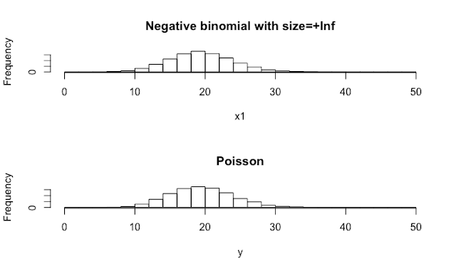
It is simple: rnbinom(n, mu=m, size=+Inf) is similar to rpois(n, lambda=m).

Try this to be sure !

layout(mat = 1:2)
x1 <- rnbinom(10000, mu=20, size =+Inf)
hist(x1, breaks=seq(from=0, to=50, by=2), main="Negative binomial with size=+Inf")
y <- rpois(10000, lambda=20)
hist(y, breaks=seq(from=0, to=50, by=2), main="Poisson")

Or this:

> dnbinom(x = 20, mu=20, size=+Inf)
[1] 0.08883532
> dpois(x=20, lambda=20)
[1] 0.08883532

Effect of size parameter, remember that size=+Inf is identical to Poisson distribution:

layout(mat = matrix(1:3, nrow= 1, byrow = TRUE))

x2 <- rnbinom(10000, mu=20, size =2)
hist(x2, breaks=seq(from=0, to=150, by=2), main="Negative binomial with size=2")

x2 <- rnbinom(10000, mu=20, size =10)
hist(x2, breaks=seq(from=0, to=150, by=2), main="Negative binomial with size=10")

x2 <- rnbinom(10000, mu=20, size =+Inf)
hist(x2, breaks=seq(from=0, to=150, by=2), main="Negative binomial with size=+Inf")

The better flexibility of the negative binomial distribution to fit counts can be seen also in my package phenology.

> library("phenology")
> 
> gr <- add_phenology(add=Gratiot, previous = NULL, month_ref = 1, format="%d/%m/%Y", name="Cayenne2001")
Cayenne2001
Reference:  2001-01-01
> 
> # fit the data using negative binomial distribution
> 
> layout(mat = matrix(1:2, nrow= 1, byrow = TRUE))
> 
> pfixed <- c(Flat=0)
> parg <- par_init(data=gr, parametersfixed = pfixed)
> parg3 <- MinBMinE_to_Min(parg)
> 
> f <- fit_phenology(data=gr, parametersfit = parg3, parametersfixed = pfixed, 
+                    trace=0, silent=TRUE)
> outf <- plot(f, main="Negative binomial")
> 
> # fit the data using Poisson distribution
> 
> pfixed <- c(Flat=0, Theta=+Inf)
> parg <- par_init(data=gr, parametersfixed = pfixed)
> parg3 <- MinBMinE_to_Min(parg)
> 
> f1 <- fit_phenology(data=gr, parametersfit = parg3, parametersfixed = pfixed, 
+                     trace=0, silent=TRUE)
> outf1 <- plot(f1, main="Poisson")
> 
> # Compare both models
> compare_AIC(Negative.binomial=f, Poisson=f1)
[1] "The lowest AIC (1350.896) is for series Negative.binomial with Akaike weight=1.000"
                       AIC DeltaAIC Akaike_weight
Negative.binomial 1350.896   0.0000  1.000000e+00
Poisson           1741.075 390.1792  1.877852e-85
> 
> # Compare the percentage of observations out of +/- 2 SD
> print("Proportion of observations out of +/- 2 SD for negative binomial distribution")
[1] "Proportion of observations out of +/- 2 SD for negative binomial distribution"
> sum((outf[[1]]$values[, "Obs"] > outf[[1]]$values[, "Theor+2SD"]) | (outf[[1]]$values[, "Obs"] < outf[[1]]$values[, "Theor-2SD"]), na.rm=TRUE) / 
+ sum(!is.na(outf[[1]]$values[, "Obs"]))
[1] 0.04383562
> 
> print("Proportion of observations out of +/- 2 SD for Poisson distribution")
[1] "Proportion of observations out of +/- 2 SD for Poisson distribution"
> sum((outf1[[1]]$values[, "Obs"] > outf1[[1]]$values[, "Theor+2SD"]) | (outf1[[1]]$values[, "Obs"] < outf1[[1]]$values[, "Theor-2SD"]), na.rm=TRUE) / 
+   sum(!is.na(outf1[[1]]$values[, "Obs"]))
[1] 0.2082192