Articles

Install raster, terra, sf or stars package in Ubuntu

To install difficult packages: raster, terra, sf or stars In terminal:  sudo apt-get install sqlite3 # sudo add-apt-repository ppa:ubuntugis/ppa && sudo apt-get update  # Provoque une erreur; pour le retirer: #  sudo apt-add-repository --remove ppa:ubuntugis/ppa Install gdal using:  sudo apt install libgdal-dev sudo apt-get install libproj-dev sudo updatedb locate libproj.so (copy the link of the file libproj.so) sudo ln -s (the link) /usr/lib/libproj.so Install libgeos: https://www.blogger.com/blog/post/edit/2061052160425746363/1945424748660662138 and sudo R install.packages("raster") install.packages("rgeos") install.packages("rgdal") install.packages("terra") install.packages("sf") install.packages("stars")

Fit a mixture of normal and lognormal distribution

Image
x.1 <-rnorm(6000, 2.4, 0.6)  x.2 <-rlnorm(10000, 1.3,0.1)    X <-c(x.1, x.2)  hist(X,100,freq=FALSE, ylim=c(0,1.5))  lines(density(x.1), lty=2, lwd=2)  lines(density(x.2), lty=2, lwd=2)  lines(density(X), lty=4)    fitnormlnorm <-function(par, val) {    p  <- 1/(1+exp(-par[5]))    return(-sum(log(p*dnorm(val, par[1], abs(par[2]), log = FALSE)+                      (1-p)*dlnorm(val, par[3], abs(par[4]), log = FALSE))))  }    # Mean 1  m1=2.3; s1=0.5  # Mean 2  m2=1.3; s2=0.1  # proportion of 1 - logit transform  p=0    par <-c(m1, s1, m2, s2, p)    result2 <-optim(par, fitnormlnorm, method="BFGS", val=X,                  hessian=FALSE, control=list(trace=1))    lines(seq(from=0, to=5, length=100),         dnorm(...

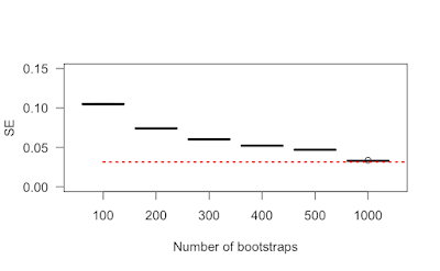
Example of bootstrap to estimate se of a set of data... just for fun

Image
N <- 1000 A <- rnorm(N) sd(A)/sqrt(N) # Vraie valeur:  1/sqrt(N) t <- NULL for (rep in rep(c(100, 200, 300, 400, 500, 1000), 10)) {   print(rep)   s <- NULL   for (i in 1:10000) {     tirage <- sample(A, size=rep, replace = TRUE)     s <- c(s, mean(tirage))   }      t <- c(t, sd(s)) } dta <- data.frame(group=rep(c(100, 200, 300, 400, 500, 1000), 10),                    mean=t) boxplot(mean ~ group, data=dta, las=1, ylab="SE", xlab="Number of bootstraps", ylim=c(0, 0.15)) segments(x0=1, x1=7, y0=1/sqrt(N), y1=1/sqrt(N), col="red", lty=3, lwd=2) In red, the true SE. The SE estimation by bootstrap is upper biased.

Get versions of R, Rstudio, shiny or packages

  The version of Rstudio can be obtained using: RStudio.Version() The running version of R is obtained by: R.version In terminal, the installed R version is obtained by: √ ~ % R --version  R version 4.3.2 (2023-10-31) -- "Eye Holes" Copyright (C) 2023 The R Foundation for Statistical Computing Platform: x86_64-pc-linux-gnu (64-bit) R is free software and comes with ABSOLUTELY NO WARRANTY. You are welcome to redistribute it under the terms of the GNU General Public License versions 2 or 3. For more information about these matters see https://www.gnu.org/licenses/. To get a package version: packageVersion(_Package name_) Other information can be found here: .libPaths() sessionInfo() For Shiny: Whitin R: system('shiny-server --version', intern = TRUE) In terminal: shiny-server --version

phantom text in graphics

Image
  The title function allows you to change the color of the text using the col argument, but that color is applied to the entire text string -- there's no obvious way to set the color of individual words. Or is there?  Barry Rowlingson offers an  elegant solution  that uses the "overhead transparency" principle of R graphics: you can overlay additional graphical elements one atop another, to build up your graph layer by layer.  So you could add the title  Hair color  in red on the left, and  Eye color  in blue on the right, and put a black "and" in the middle.  The trick is in the positioning -- it could take a lot of trial and error to get the  x  position of each element correct.  But if you plot the same text three times in three different colors, but leave some words blank (so they won't overlay previously plotted elements) you don't have to worry about positioning at all.  The  phantom  notation allows y...

Force system messages to be in English

 > warning("Essai") Message d'avis : Essai  > Sys.setenv(LANG = "en") > warning("Essai") Warning message: Essai 

Distribution when only quantiles are known

Imagine that you have a credible interval (0.01, 0.3) for (0.025, 0.975) probabilities for one proportion value and you would like to use this variable. The solution is to search for the beta distribution that gives this credible interval: library("HelpersMG") best <- fitdistrquantiles(quantiles = c(0.01, 0.3), probs=c(0.025, 0.975), scaled=FALSE, distribution = "beta") Then it is possible to try the result: rd10000 <- rbeta(10000, shape1 = best["shape1"], shape2 = best["shape2"]) quantile(rd10000, probs=c(0.025, 0.975)) It works ! This function can fit also more than 2 quantiles and can be used for gamma and normal distributions. Now let do a simple exercise Let p and q two independent proportions being known only from their confidence interval and median: p <- c("2.5%"=0.012, "50%"=0.14, "97.5%"=0.25) q <-  c("2.5%"=0.37, "50%"=0.52, "97.5%"=0.75) I want the confidence inte...