Articles

Affichage des articles du décembre, 2019

Generate random distribution of truncated distribution

Imagine that you have estimated a sex ratio being 0.8 SE 0.2 by maximum likelihood. If you want make an histogram showing this distribution, the first idea is to do: > sr <- rnorm(100000, mean=0.8, sd=0.2) > sd(sr) [1] 0.2001526 > hist(sr) > sum(sr>1) [1] 15680 > sum(sr<0) [1] 3 The sd of sr is right 0.2 but clearly, it is not correct ! Let do a truncation: > sr <- sr[(sr>0) & (sr<1)] > hist(sr) > length(sr) [1] 84317 > sd(sr) [1] 0.1591352 The histogram is correct but the standard deviation is less than 0.2 due to the truncation. > sfinal <- NULL > x <- seq(from=1E-6, to=1, length.out = 100) > for (sigma in x) +   sfinal <- c(sfinal, abs(sd(sin(rnorm(100000, mean=2*asin(sqrt(0.8)), sd=sigma)/2)^2) - 0.2)) > plot(x, sfinal, type="l") > sigma <- x[which.min(sfinal)] > distribution_sr <- sin(rnorm(100000, mean=2*asin(sqrt(0.8)), sd=sigma)/2)^2 > hist(distribution_s...
Variance of combination of variables

m1 <- 10 v1 <- 2 m2 <- 100 v2 <- 5 # var(x + y) = var(x) + cov(x, y) + var(y) # if the x and y variables are independent: # var(x + y) = var(x) + var(y) (v1 + v2) # If I use resampling c1 <- rnorm(100000, mean=m1, sd=sqrt(v1)) c2 <- rnorm(100000, mean=m2, sd=sqrt(v2)) var(c1+c2) # The resampling method can be used in most of the cases

Makevars

In ~/.r (base) marcgirondot@MacBook-Air-de-Marc .r % cat Makevars # The following statements are required to use the clang4 binary CC=/usr/local/opt/llvm/bin/clang CXX=/usr/local/opt/llvm/bin/clang CXX11=/usr/local/opt/llvm/bin/clang CXX14=/usr/local/opt/llvm/bin/clang CXX17=/usr/local/opt/llvm/bin/clang CXX1X=/usr/local/opt/llvm/bin/clang          LDFLAGS=-L/usr/local/opt/llvm/lib # End clang4 inclusion statements

system variable within R

To let R know about the compiler, we need to modify the ~/.Renviron. You may need to create the file by running in Terminal (Applications -> Utilities): touch ~/.Renviron Then, inside of ~/.Renviron add: PATH="/usr/local/clang7/bin:${PATH}" See http://thecoatlessprofessor.com/programming/r-compiler-tools-for-rcpp-on-macos/

Install previous version of a package

(the problem is solved with raster package; I keep this publication to show how to install previous version of a package) require(devtools) install_version("raster", version = "2.5-8", repos = " http://cran.us.r-project.org ")

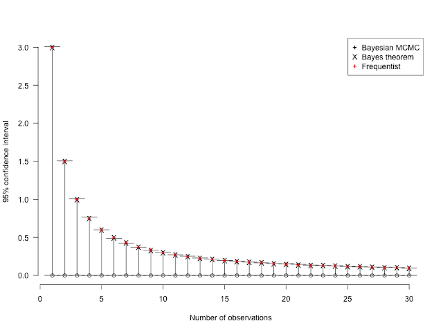
Confidence interval of 0 observations with Poisson distribution

Image
https://stats.stackexchange.com/questions/427019/confidence-interval-for-mean-of-poisson-with-only-zero-counts Excellent answer in this link about the confidence interval when only 0 observations are available for a Poisson distribution. Here is an alternative using Bayesian MCMC with uniform distribution. This is surprising how close are the estimates ! library(HelpersMG) u <- NULL for (l in 1:30) {   val <- rep(0, l)   prior <- data.frame(Density="dunif",                       Prior1=0, Prior2=10,                       SDProp=1,                       Min=0, Max=10,                       Init=0.01, row.names = "lambda")   mcmc_run <- MHalgoGen(n.iter=100000, parameters=prior, data=val, adaptive = TRUE,     ...

Install mark and RMark in Ubuntu 18.04

Enter this in terminal, and after you can install the package Rmark: cd /usr/local/bin sudo wget -U "Mozilla/5.0 (Macintosh; Intel Mac OS X 10_9_3) AppleWebKit/537.75.14 (KHTML, like Gecko) Version/7.0.3 Safari/7046A194A" http://www.phidot.org/software/mark/downloads/files/mark.64.zip sudo unzip mark.64.zip sudo rm mark64.zip sudo rm mark64.static sudo cp mark64.dynamic mark sudo rm mark64.dynamic sudo chmod +x mark sudo apt-get install libgfortran5 And in R: install.packages("RMark")

Regroup daily history for Rmark analysis

If you have daily CMR data, it can be too huge information for CMR analysis using Rmark. A solution is to group data by time period. Here is a solution without using any for loop. regrouphistory <- function(history, group=7) { if (any(sapply(history, nchar)!=nchar(history[1]))) stop("All histories must be of the same length") h1 <- strsplit(history, "") factor <- as.character(1:((length(h1[[1]]) %/% group)+1)) f <- as.character(sapply(factor, FUN=function(x) rep(x, group)))[seq_along(h1[[1]])] r <- sapply(h1, function(h) {h3 <- vapply(split(h, f), function(x) ifelse(any(x=="1"), "1", "0"), FUN.VALUE = "0") h3 <- h3[order(as.numeric(names(h3)))] return(paste0(h3, collapse = "")) }) return(r) } histoire <- "000000001000010100000100000100001000000000000" regrouphistory(histoire, group=10) [1] "11110" histoire <- c("0000000010000101000001000001000010...

Install mark in MacOSX

brew tap sjbonner/tap brew install mark-on-mac Done !

ifelse() must be used with caution

The if else statement is very useful when you work with a vector, but take care, it must be used with caution because it can be very slow : Aini =  runif(1000000, min=-1,max=1) library(microbenchmark) A <- Aini microbenchmark({B1 <- ifelse( A < 0, sqrt(-A), A )}) # mean = 77.55551 A <- Aini microbenchmark({B2 <- ifelse( A < 0, suppressWarnings(sqrt(-A)), A )}) # mean = 76.53762 A <- Aini microbenchmark({B3 <- ifelse( A < 0, sqrt(abs(A)), A )}) # mean = 75.26712 A <- Aini microbenchmark({A[A < 0] <- sqrt(-A[A < 0]);B4 <- A}) # mean = 17.71883

Understanding glm

Let do a simple glm to explore exactly how it works: > datax <- data.frame(y=rnorm(100), x1=rnorm(100), +                     x2=rnorm(100), x3=rnorm(100), x4=rnorm(100),  +                     x5=sample(x=c("A", "B"), size=100, replace = TRUE)) > gnul <- glm(y ~ 1, data=datax) First, let see the number of fitted parameters : > length(gnul$coefficients) [1] 1 But when you use logLik(), two parameters are indicated as df=: > logLik(gnul) 'log Lik.' -153.8374 (df=2) If you do the glm "by hand", the number of fitted parameters is 2: > dnormx <- function(x, data) {-sum(dnorm(data, mean=x["mean"], sd=x["sd"], log = TRUE))} > parg <- c(mean=0, sd=1) > o0 <- optim(par = parg, fn=dnormx, data=datax[, "y"]) > o0$par       mean         sd  -0.1338348  1.1270446  > o0$value [1] 153...

AIC for mixed models: cAIC

Model selection was performed using the conditional Akaike information criterion (cAIC). This measure of the quality of fit penalised by the number of parameters corrected (Burnham and Anderson, 2002) was specially developed for mixed models (Greven and Kneib, 2010; Säfken et al., 2018 preprint). Greven S, Kneib T (2010) On the behaviour of marginal and conditional Akaike Information Criteria in linear mixed models. Biometrika 97: 773-789 Säfken B, Rügamer D, Kneib T, Greven S (2018) Conditional model selection in mixed-effects models with cAIC4. arXiv 1803.05664v2: 1-31 library(cAIC4) datax <- data.frame(y=rnorm(100), x1=rnorm(100),                     x2=rnorm(100), x3=rnorm(100), x4=rnorm(100), x5=sample(x=c("A", "B"), size=100, replace = TRUE)) g0 <- lmer(y ~ x1+x2+x3+x4 + (1 | x5), data=datax) cAIC(g0) cAIC(g0)$caic

clang in Macosx

By default, the clang version used is the one provided by Xcode (base) marcgirondot@MacBook-Air-de-Marc bin % clang --version Apple clang version 11.0.0 (clang-1100.0.33.12) Target: x86_64-apple-darwin19.0.0 Thread model: posix InstalledDir: /Applications/Xcode.app/Contents/Developer/Toolchains/XcodeDefault.xctoolchain/usr/bin If you install gcc using homebrew, you have another version: (base) marcgirondot@MacBook-Air-de-Marc bin % /usr/local/opt/llvm/bin/clang --version clang version 9.0.0 (tags/RELEASE_900/final) Target: x86_64-apple-darwin19.0.0 Thread model: posix InstalledDir: /usr/local/opt/llvm/bin The Xcode version of clang does not understand the option -fopenmp whereas the version of gcc understand this option. Then it can be important to know which version of clang you are using. You can define which clang version to be used in R session by setting: ~/.R/Makevars with # The following statements are required to use the clang...